Chapter 7 Topology and Geocoding
Frequently, we need spatial data to behave and relate and in specific and predictable ways. Many types of analyses may expect spatial data to be represented and interact in a standard form. In this chapter, we will extend our knowledge of data models using topology, which unlocks many advanced spatial analyses. We will look at a specific example of an analysis that requires topology, geocoding, which will be a convenient segue into network analysis discussed in the following chapter.
Learning Objectives
- Understand the role of topology in governing data behaviour
- Recognize some examples and uses of 2D topologies
- Practice solving topological errors
- Identify spatial data models that support topology
- Understand the process of geocoding
- Practice geocoding addresses and reverse geocoding addresses to other coordinate systems
- Analyze attributes of census data
Key Terms
Vertex, Node, Pseudonode, Dangle, Planar Topology, Non-Planar Topology, Geocoding, Adjacency, Overlap, Connect, Inside, Reverse Geocoding, small change
7.1 Topology
Topology describes the relationships of spatial data. This is a very broad definition that encompasses the wide range of possible arrangements of spatial data in practice. If we drill down into this concept, topology is really what allows us undertake specific types of analysis that requires or expects spatial data to behave in a certain way. If you think about the feature geometries that we have at our disposal, then there are no fewer than nine combinations of how these geometries can interact as illustrated in Figure 7.1 below.
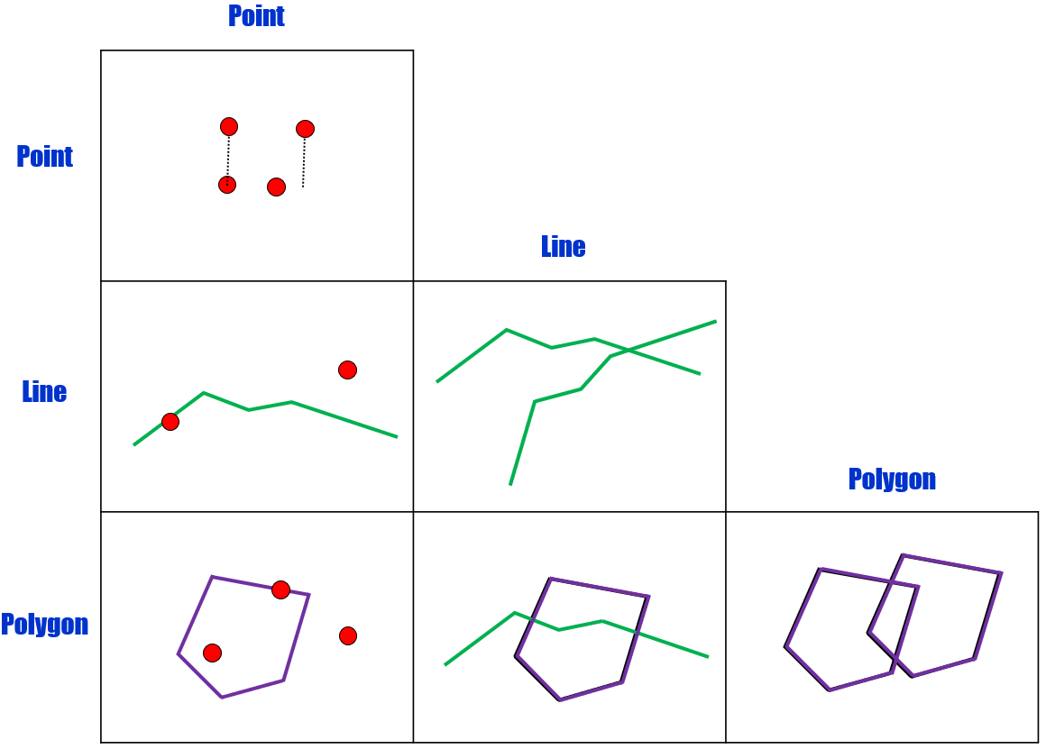
Figure 7.1: Grid showing all the combinations of how point, line and polygon geometries can interact. Pickell, CC-BY-SA-4.0.
It is important to recognize that there may be cases where we “expect” that a given combination of features will conform to a specific interaction. For example, the provinces and territories of Canada are typically represented as polygons that share adjacent boundaries. That is, the adjacent boundaries shared between any two provinces or territories cannot logically overlap as this representation (model) would contravene the legal definitions of the provinces and territories. In another case, a human technician may erroneously digitize a road that crosses another road without indicating that the two roads share an intersection, which could have consequences for how traffic flow can be modeled between the two roads (i.e., intersection with traffic light versus overpass). These are both examples of situations where topology is needed. Topology applies logic to define how features are expected to relate to other features in order to conform to knowledge systems like legal definitions of land and traffic flow. In short, topology ensures data integrity for other types of analysis.
7.2 Planar vs. Non-Planar Topology
In the context of topology, planar refers to the concept that all vertices of feature vector geometry are mapped onto the same plane. So in a planar world-view, all lines and polygons share coincident vertices. For example, if two polygons overlap, then the overlapping area forms a new polygon with a boundary of vertices defined by the union of the two other polygons. Also, if two lines overlap, then the two lines are divided into four new segments and a new vertex is formed at the intersection. In other words, planar topology does not allow polygons or lines to lay “underneath” or “on top” of another line or polygon and feature geometries must always be distinct.
On the other hand, non-planar topology is the concept that vertices of feature vector geometry can be mapped to different planes. It is important to emphasize here that when we are talking about planes that we are not referring to projected coordinate systems. It is generally assumed that any two spatial data layers containing feature geometries are interacting within the same projected coordinate system. Non-planar topology allows for other knowledge systems to be represented in spatial data. The case where a pipeline runs underneath a river or a territory that was traditionally used by several Indigenous peoples (Figure 7.2) are examples of valid non-planar topology.
## Warning: package 'leaflet' was built under R version 4.1.1## Warning: package 'rgdal' was built under R version 4.1.1## Loading required package: sp## Warning: package 'sp' was built under R version 4.1.2## Please note that rgdal will be retired by the end of 2023,
## plan transition to sf/stars/terra functions using GDAL and PROJ
## at your earliest convenience.
##
## rgdal: version: 1.5-27, (SVN revision 1148)
## Geospatial Data Abstraction Library extensions to R successfully loaded
## Loaded GDAL runtime: GDAL 3.2.1, released 2020/12/29
## Path to GDAL shared files: C:/Users/User/Documents/R/win-library/4.1/rgdal/gdal
## GDAL binary built with GEOS: TRUE
## Loaded PROJ runtime: Rel. 7.2.1, January 1st, 2021, [PJ_VERSION: 721]
## Path to PROJ shared files: C:/Users/User/Documents/R/win-library/4.1/rgdal/proj
## PROJ CDN enabled: FALSE
## Linking to sp version:1.4-5
## To mute warnings of possible GDAL/OSR exportToProj4() degradation,
## use options("rgdal_show_exportToProj4_warnings"="none") before loading sp or rgdal.
## Overwritten PROJ_LIB was C:/Users/User/Documents/R/win-library/4.1/rgdal/projgetTilesURL <- "https://tile.thunderforest.com/landscape/{z}/{x}/{y}.png?apikey=06d706f23fc4461db5db742f930174fc"
m <- leaflet(native_land) %>%
addTiles(getTilesURL) %>%
addScaleBar(position = c("topleft")) %>%
setView(lat = 49.25, lng = -125, zoom = 7) %>%
addPolygons(data=native_land,
fillColor = native_land@data$color,
weight = 0.6,
opacity = 0.5,
color = "#ffffff",
dashArray = NULL,
fillOpacity = 0.25,
highlight = highlightOptions(
weight = 1.8,
color = "#7d7d7d",
dashArray = NULL,
fillOpacity = 0.7,
bringToFront = TRUE),
label = labels,
labelOptions = labelOptions(
style = list("font-weight" = "normal", padding = "3px 8px"),
textsize = "12px", direction = "auto"))Figure 7.2: Non-planar topology of 36 indigenous territories overlapping Vancouver Island, British Columbia. Data from contributors at native-land.ca, CC0.
7.3 Implementing Planar Topology
Implementing planar topology involves defining specific rules for how features should relate to one another given some analytical context. This process also requires that the spatial data are housed a relational database or data model that supports topology. In other words, topology is enforced only by data models that support topological rules. When a topological rule is violated, the relational database identifies the contravening features and displays them on the map and in the attribute table. Then, it is up to an expert GIS technician to decide how the error should be corrected. For example, some errors like intersecting lines can automatically be split at the intersection while overlapping polygons might need to be manually edited to reflect the correct adjacency. Thus, the process of applying topology is first to work within a data model that supports topology, then choose the topological rules that reinforce a particular knowledge system, and finally to inspect and decide how to deal with any contraventions. Since planar topology is only supported by certain data models, and some data models are proprietary to certain software, the exact topological rules that can be implemented in a GIS are mostly dependent on the software that you are using. Instead of examining a specific GIS software package, we will discuss the “fundamental” planar topological relationships that are common across nearly all implementations of topology. (If you want to know more about how topology is implemented within specific data models, skip ahead to the “Data models supporting planar topology” section.)
So far, we have seen that there are six ways to combine feature geometries (points, lines, and polygons). We can extend this understanding to include at least six different ways that they can relate to one another: adjacent; overlap; intersect; connect; cover; and inside. Some of these relationships can be modeled between two different spatial layers (e.g., two point layers) or within a single spatial layer. In the following sections, we will look at different planar topological rules that apply both between and within feature geometries.
7.4 Adjacency and Overlap
There are times when we need to ensure that two polygons are adjacent to one another by sharing a common edge. If two polygons are not adjacent to one another, then a gap, known as a sliver, exists between them or they must overlap. Consider the case where we are mapping land covers. If we have a formal scheme that describes all possible land covers, then we expect that a map of land covers will have perfect adjacency between all polygons so that there are no areas that are not mapped (i.e., slivers) and that no area has multiple, overlapping land covers. Since lines are also 2-dimensional, lines can overlap other lines. Depending on the context, a topological rule may be needed to promote or prevent this relationship. For example, if you are modeling bus routes, then one road might support several different routes.
[figure of sliver] [figure of overlap]
Some examples of adjacency and overlap topological rules: - Polygons within the same layer must not have gaps - Polygons within the same layer must not overlap - Polygons must not overlap other polygons - Lines must not overlap other lines - Lines must not self-overlap
7.5 Intersect and Connect
As we have seen from Chapter 3, lines are often used to represent phenomena that flow, so intersection and connection are important concepts for these representations. Important to understanding how connection and intersection work in planar topology, we need to understand that lines are comprised of a set of vertices and nodes. A node is simply the terminating vertex in a set of vertices for a line. For example, suppose the line segment \(A\) has a set of vertices, \([[1,0],[1,3],[1,5]]\). Then the nodes for \(A\) are \([1,0]\) and \([1,5]\) (Figure 7.3). Since nodes define the end points of a line segment, they are key to enforcing connection rules. We will look at network analysis in more detail in the next chapter. For now, let us consider two different networks that can help us conceptualize some fundamental line topology using nodes.
fig_cap <- paste("Lines are always comprised of two nodes. Line A shown here has nodes at [1,0] and [1,5]. Pickell, CC-BY-SA-4.0.")
Ax <- c(1,1,1)
Ay <- c(0,3,5)
plot(1,1,ylim=c(-1,6),xlim=c(-1,6),type="n",xlab="",ylab="",xaxt="n",yaxt="n")
axis(1,at=-1:6)
axis(2,at=-1:6)
abline(h=-1:6,v=-1:6,col="grey")
lines(Ax,Ay,type="o",lwd=2,pch=19,col="#7b3294")
labs <- c("(1,0)","(1,3)","(1,5)")
text(Ax,Ay-0.2,labels=labs, cex=0.9, font=2, pos=4,col="#7b3294")
text(0.75,2.5,"A", cex=1, font=2,col="#7b3294")![Lines are always comprised of two nodes. Line A shown here has nodes at [1,0] and [1,5]. Pickell, CC-BY-SA-4.0.](open-geomatics-textbook_files/figure-html/7-node-1.png)
Figure 7.3: Lines are always comprised of two nodes. Line A shown here has nodes at [1,0] and [1,5]. Pickell, CC-BY-SA-4.0.
A network of streams and rivers is based on the hydrological knowledge system that explains how water moves over a terrain surface. In both theory and practice, we know that water flows from higher elevations to lower elevations with limited exceptions. Thus, we expect that streams will connect with other streams and continue to flow towards some outlet such as an ocean. Connection refers to the fact that the endpoint node of one stream will fall somewhere on another stream segment. Where two line segments come together, it is possible for one segment \(A\) to “undershoot” the other segment \(B\), resulting in the end node of segment \(A\) appropriately named a dangle Figure 7.4) and a loss of connection.
fig_cap <- paste("A dangle forms when a line (B) does not connect to another line (A). Pickell, CC-BY-SA-4.0.")
Ax <- c(1,1,1)
Ay <- c(0,3,5)
Bx <- c(2,4)
By <- c(2,2)
plot(1,1,ylim=c(-1,6),xlim=c(-1,6),type="n",xlab="",ylab="",xaxt="n",yaxt="n")
axis(1,at=-1:6)
axis(2,at=-1:6)
abline(h=-1:6,v=-1:6,col="grey")
lines(Ax,Ay,type="o",lwd=2,pch=19,col="#7b3294")
lines(Bx,By,type="o",lwd=2,pch=19,col="#008837")
labs <- c("(1,0)","(1,3)","(1,5)")
text(Ax,Ay-0.2,labels=labs, cex=0.9, font=2, pos=4,col="#7b3294")
labs <- c("(2,2)","(4,2)")
text(Bx,By-0.2,labels=labs, cex=0.9, font=2, pos=4,col="#008837")
text(0.75,2.5,"A", cex=1, font=2,col="#7b3294")
text(3.5,2.5,"B", cex=1, font=2,col="#008837")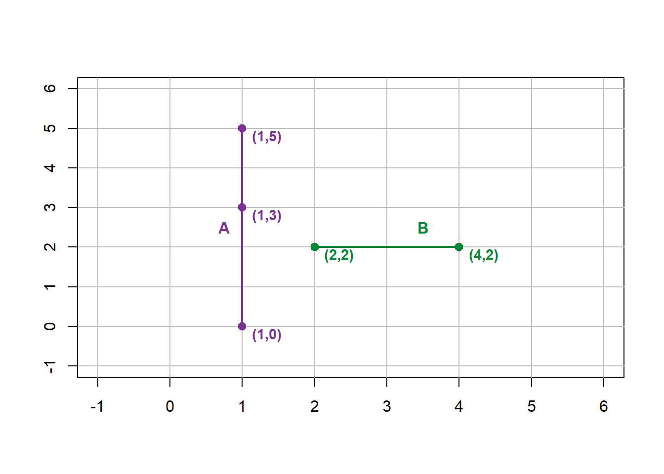
Figure 7.4: A dangle forms when a line (B) does not connect to another line (A). Pickell, CC-BY-SA-4.0.
Dangles are the opposite case to intersections, which occur when two line segments cross each other. With planar topology, intersections must be modeled with a shared node representing the intersection location. For example, suppose line segment \(B\) has a set of vertices, \([[0,1],[2,1],[4,1]]\). If line segments \(A\) (defined above) and \(B\) are mapped together with non-planar topology, then they will intersect at \([1,2]\), which is not a vertex represented in either segment (Figure 7.5).
fig_cap <- paste("Line A mapped with Line B in non-planar topology. Pickell, CC-BY-SA-4.0.")
Ax <- c(1,1,1)
Ay <- c(0,3,5)
Bx <- c(0,2,4)
By <- c(2,2,2)
plot(1,1,ylim=c(-1,6),xlim=c(-1,6),type="n",xlab="",ylab="",xaxt="n",yaxt="n")
axis(1,at=-1:6)
axis(2,at=-1:6)
abline(h=-1:6,v=-1:6,col="grey")
lines(Ax,Ay,type="o",lwd=2,pch=19,col="#7b3294")
lines(Bx,By,type="o",lwd=2,pch=19,col="#008837")
labs <- c("(1,0)","(1,3)","(1,5)")
text(Ax,Ay-0.2,labels=labs, cex=0.9, font=2, pos=4,col="#7b3294")
labs <- c("(0,2)","(2,2)","(4,2)")
text(Bx,By-0.2,labels=labs, cex=0.9, font=2, pos=4,col="#008837")
text(0.75,2.5,"A", cex=1, font=2,col="#7b3294")
text(3.5,2.5,"B", cex=1, font=2,col="#008837")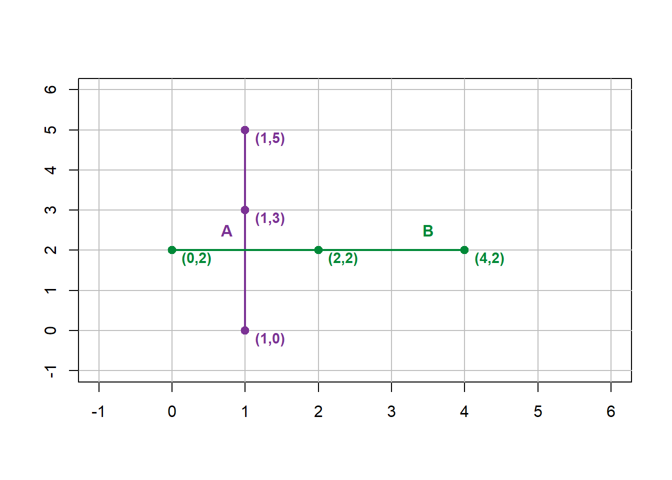
Figure 7.5: Line A mapped with Line B in non-planar topology. Pickell, CC-BY-SA-4.0.
Thus, the intersection of \(A\) and \(B\) with planar topology would yield four new segments: \(C=[[0,2],[1,2]]\), \(D=[[1,2],[1,3],[1,5]]\), \(E=[[1,2],[2,2],[4,2]]\), and \(F=[[1,0],[1,2]]\). Figure 7.6 illustrates how all four of these new segments share the same node \([1,2]\) at the intersection of \(A\) and \(B\).
fig_cap <- paste("Line A mapped with Line B in planar topology yields segments C, D, E, and F. All segments share (1,2) as a node. Pickell, CC-BY-SA-4.0.")
Cx <- c(0,1)
Cy <- c(2,2)
Dx <- c(1,1,1)
Dy <- c(2,3,5)
Ex <- c(1,2,4)
Ey <- c(2,2,2)
Fx <- c(1,1)
Fy <- c(0,2)
plot(1,1,ylim=c(-1,6),xlim=c(-1,6),type="n",xlab="",ylab="",xaxt="n",yaxt="n")
axis(1,at=-1:6)
axis(2,at=-1:6)
abline(h=-1:6,v=-1:6,col="grey")
lines(Cx,Cy,type="o",lwd=2,pch=19,col="#e41a1c")
lines(Dx,Dy,type="o",lwd=2,pch=19,col="#377eb8")
lines(Ex,Ey,type="o",lwd=2,pch=19,col="#f781bf")
lines(Fx,Fy,type="o",lwd=2,pch=19,col="#ff7f00")
labs <- c("(0,2)","")
text(Cx,Cy-0.2,labels=labs, cex=0.9, font=2, pos=4,col="#e41a1c")
labs <- c("","(1,3)","(1,5)")
text(Dx,Dy-0.2,labels=labs, cex=0.9, font=2, pos=4,col="#377eb8")
labs <- c("","(2,2)","(4,2)")
text(Ex,Ey-0.2,labels=labs, cex=0.9, font=2, pos=4,col="#f781bf")
labs <- c("(1,0)","")
text(Fx,Fy-0.2,labels=labs, cex=0.9, font=2, pos=4,col="#ff7f00")
text(0.5,2.5,"C", cex=1, font=2,col="#e41a1c")
text(0.75,4.5,"D", cex=1, font=2,col="#377eb8")
text(3.5,2.5,"E", cex=1, font=2,col="#f781bf")
text(0.75,0.5,"F", cex=1, font=2,col="#ff7f00")
points(1,2,pch=19)
text(1,2-0.2,"(1,2)",pos=4,font=2,cex=0.9)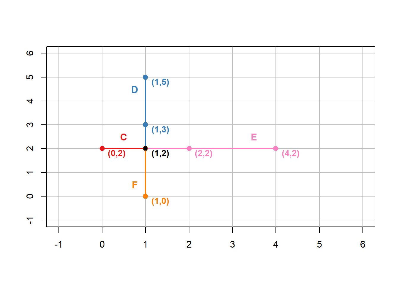
Figure 7.6: Line A mapped with Line B in planar topology yields segments C, D, E, and F. All segments share (1,2) as a node. Pickell, CC-BY-SA-4.0.
As well, pseudonodes can occur when a node does not actually terminate a line segment at a junction, for example, between two streams or roads. In other words, a pseudonode is a node that is shared by two lines. Figure 7.7 illustrates a pseudonode occurring at \([3,5]\).
fig_cap <- paste("Lines A and B share a pseudonode at [3,5], indicated in red. Pickell, CC-BY-SA-4.0.")
Ax <- c(0,1,3)
Ay <- c(0,3,5)
Bx <- c(3,4,3)
By <- c(5,3,1)
plot(1,1,ylim=c(-1,6),xlim=c(-1,6),type="n",xlab="",ylab="",xaxt="n",yaxt="n")
axis(1,at=-1:6)
axis(2,at=-1:6)
abline(h=-1:6,v=-1:6,col="grey")
lines(Ax,Ay,type="o",lwd=2,pch=19,col="#7b3294")
labs <- c("(0,0)","(1,3)","(3,5)")
text(Ax,Ay-0.2,labels=labs, cex=0.9, font=2, pos=4,col="#7b3294")
text(0.5,3.5,"A", cex=1, font=2,col="#7b3294")
lines(Bx,By,type="o",lwd=2,pch=19,col="#008837")
labs <- c("(3,5)","(4,3)","(3,1)")
text(Bx,By-0.2,labels=labs, cex=0.9, font=2, pos=4,col="#008837")
text(3.5,3,"B", cex=1, font=2,col="#008837")
points(3,5,col="red",pch=19)![Lines A and B share a pseudonode at [3,5], indicated in red. Pickell, CC-BY-SA-4.0.](open-geomatics-textbook_files/figure-html/7-pseudonode-1.png)
Figure 7.7: Lines A and B share a pseudonode at [3,5], indicated in red. Pickell, CC-BY-SA-4.0.
Some examples of intersection and connection topological rules: - Lines must not intersect other lines - Lines must intersect other lines - Lines must not self-intersect - Lines within a same layer must not self-intersect - Lines must not have dangles
7.6 Coincident and Disjoint
Point features can be either coincident or disjoint with other point features. Point features that need to be disjoint may be representing trees, mountain peaks, or any similar type of feature that would be expected to be discrete in geographic space. There are also instances where we might need one set of point features to be coincident with another such as field plots that are centered using a tree or other spatially-discrete feature on the landscape.
Some examples of coincident and disjoint topological rules: - Points must be disjoint with other points - Points must by coincident with other points
7.7 Cover
Cover refers to planar topology where a feature lays on or within another feature. For example, dams represented as point features must be covered by a line representing a river (Figure 7.8). Similarly, lines representing rivers must be covered by polygons representing watersheds. As well, property parcel polygons must be covered by the municipal or regional tax authority polygon.
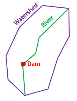
Figure 7.8: Topological relationship between dam (point) covered by a river (line), which is covered by a watershed (polygon). Pickell, CC-BY-SA-4.0.
Some examples of cover topological rules: - Point must be covered by a line - Point must be covered by a polygon - Line must be covered by a polygon - Polygon must be covered by a polygon
7.7.1 Multipart geometries
Sometimes we need to represent several points, lines or polygons as a collection, which is known as multipart geometries. Multipart geometries allow us to represent several disjoint and non-adjacent geometries as a single feature. In this way, we can assign attribute values to the collection of features rather than each geometry individually. The territorial boundary of Canada is a good example of an instance where a multipart geometry can be useful because all of the contiguous land and non-contiguous land (i.e., islands) can be represented and associated with a single feature in the attribute table. However, if the distinction of features is important, such as identifying the names of islands in the Haida Gwaii archipelago, then a singlepart geometry should be used (Figure 7.9).
Figure 7.9: Singlepart geometry of the Haida Gwaii archipelago off the west coast of British Columbia, Canada. Hover over the islands to see the names. Polygon data from Statistics Canada and island placenames from Natural Resources Canada. Open Government License - Canada.
Although it is possible to convert from a multipart geometry into singlepart geometries, you need to carefully consider how your features should be represented in the attribute table. For example, if you will be undertaking calculations using area or perimeter of the constituent polygons that comprise a multipart geometry of Canada, then you will return a single value for all of Canada while singlepart geometries would return values for each individual polygon. As well, area calculations can vary depending on the model you use. For example, approximately 27% of Canada’s land area (including freshwater), is comprised of more than 52,000 islands, which is a statistic you could only calculate with singlepart geometry. Thus, the choice of representing a feature using singlepart or multipart geometry should be based on how the features will be used in your analysis (i.e., aggregated versus disaggregated).
7.8 3D topologies
7.8.1 Multipatch geometries
Like multipart geometries, multipatch geometries represent several faces of a 3D feature such as a building or tree. Since 3D objects are comprised of several polygon faces, these 2D geometries must be referenced to the same feature in order to enforce topological rules.
7.8.2 Convex hull
7.8.3 Delauney triangles
7.8.4 Data models supporting planar topology
7.9 Geocoding
Geocoding is the process of converting addresses to geographic coordinates, while reverse geocoding is the process of converting geographic coordinates to addresses (Figure ??). In order to achieve this conversion, an address locator uses reference spatial data that are mapped to a geographic or projected coordinate system in order to locate new addresses or coordinates. Usually, an address locator relies on several pieces of reference spatial data such as maps of road networks, postal codes, cities, provinces or states, and countries. If you It is important that the city, province, and country are mapped and specified because road names frequently repeat in different cities (e.g., Main Street). If you are aiming to geocode addresses in a single city, then it is feasible to manually specify your own address locator using available data such as roads, parcels, neighborhoods, and postal codes. However, for geocoding across large areas, this may not be feasible and you should instead rely on geocoding services that use large databases of reference spatial data.
7.10 Geocoding Services
7.11 Case Study: Working with Canadian Census Data
7.12 Summary
Lorem ipsum dolor sit amet, consectetur adipiscing elit. Ut in dolor nibh. Lorem ipsum dolor sit amet, consectetur adipiscing elit. Praesent et augue scelerisque, consectetur lorem eu, auctor lacus. Fusce metus leo, aliquet at velit eu, aliquam vehicula lacus. Donec libero mauris, pharetra sed tristique eu, gravida ac ex. Phasellus quis lectus lacus. Vivamus gravida eu nibh ac malesuada. Integer in libero pellentesque, tincidunt urna sed, feugiat risus. Sed at viverra magna. Sed sed neque sed purus malesuada auctor quis quis massa.
Reflection Questions
- Give some examples of situations where you might use planar and non-planar
- Define ipsum lorem.
- What is the role of ispum lorem?
- How does ipsum lorem work?
Practice Questions
- Draw a convex hull for the points below.
- Given ipsum, solve for lorem.
- Draw ipsum lorem.
Recommended Readings
Ensure all inline citations are properly referenced here.