Chapter 10 Fundamentals of remote sensing
At some point in your life you may have wondered why the sky is blue. You may have noticed that two leaves on the same tree are slightly different shades of green. It would be perfectly natural to wonder these things and simply allow the questions to remain unanswered. After all, they likely carry minimal significance compared to the other queries of your life. What if, however, these questions could not only be answered, but also lead you to profound insights relating to your environment? What if differences in leaf color indicated an early summer drought or the initial stages of a pest outbreak that would wreak havoc on the economy? Remote sensing is the overarching term that refers any scientific exploration that seeks to address these, and many other questions.
Learning Objectives
- Understand key principles underpinning remote sensing science
- Become familiar with specific types of energy used in RS
- Define key interactions between energy and surface materials that enable RS
- Comprehend various considerations that effect the use of RS
Key Terms
Radiation, Energy, Photons, Electromagnetic Spectrum, Wavelength, Resolution, Raster, Image, Pixel
10.1 What is remote sensing?
Simply put, remote sensing is any method of gathering information about an object, or objects, without physical contact. Over the course of human history, a variety of remote sensing techniques have been used. In fact, one could argue that any organism capable of observing electromagnetic radiation has a built in optical remote sensing system, such as human vision. Similar arguments could be made for other senses, such as smell or hearing, but this chapter will focus strictly on techniques that capture and record electromagnetic radiation.
One of the first recorded conceptualizations of remote sensing was presented by Plato in the Allegory of a Cave, where he philosophized that the sense of sight is simply a contracted version of reality from which the observer can interpret facts presented through transient images created by light (Allegory of a Cave). Over the next few centuries a variety of photosensitive chemicals were discovered which enabled the transient images humans see to be recorded . This technology was called photography (see A History of Photography). The ability to record the interaction of light and specific objects within a scene proved enabled the preservation of information in an accessible medium. Eventually, photography became a prominent means of immortalizing everything from individual humans to exotic landscapes. After all, a picture says a thousand words.
In 1858, an enthusiastic Frenchman named Gaspard Tournachon mounted a camera on a hot air balloon and captured images of the earth below him. These images were taken as the camera looked down at a small village outside Paris. For the first time it was possible to examine the distribution of buildings, fields, forests and roads across the landscape. With this, airborne remote sensing was born. Remote sensing technologies continued to advance throughout the 19th and 20th centuries, with major socio-political conflicts like World War I and II acting as crucibles for innovation. The advancement of remote sensing has continued into the 21st century and is unlikely to slow down in the future. This is due to the relevance of three key aspects.
First and foremost, remote sensing enables the observation of objects in, or from, locations that are otherwise inaccessible for humans. The observation of Mars’ surface from an orbiting satellite is a one current example. A second aspect that makes remote sensing so useful is the collection of information over a large area. For example, airborne remote sensing technologies enable observations of land cover across Canada (Figure 10.1). The ability to evaluate inaccessible objects or large areas over time is a third valuable aspect of remote sensing and is particularly relevant for land management, as predictions can be informed through the observation of historic patterns and processes. This is especially true for projects aiming to restore degraded ecosystems or plan sustainable land use practices. Before exploring the designs of specific sensor or their applications, however, it is essential to grasp some key components that underpin remote sensing science.
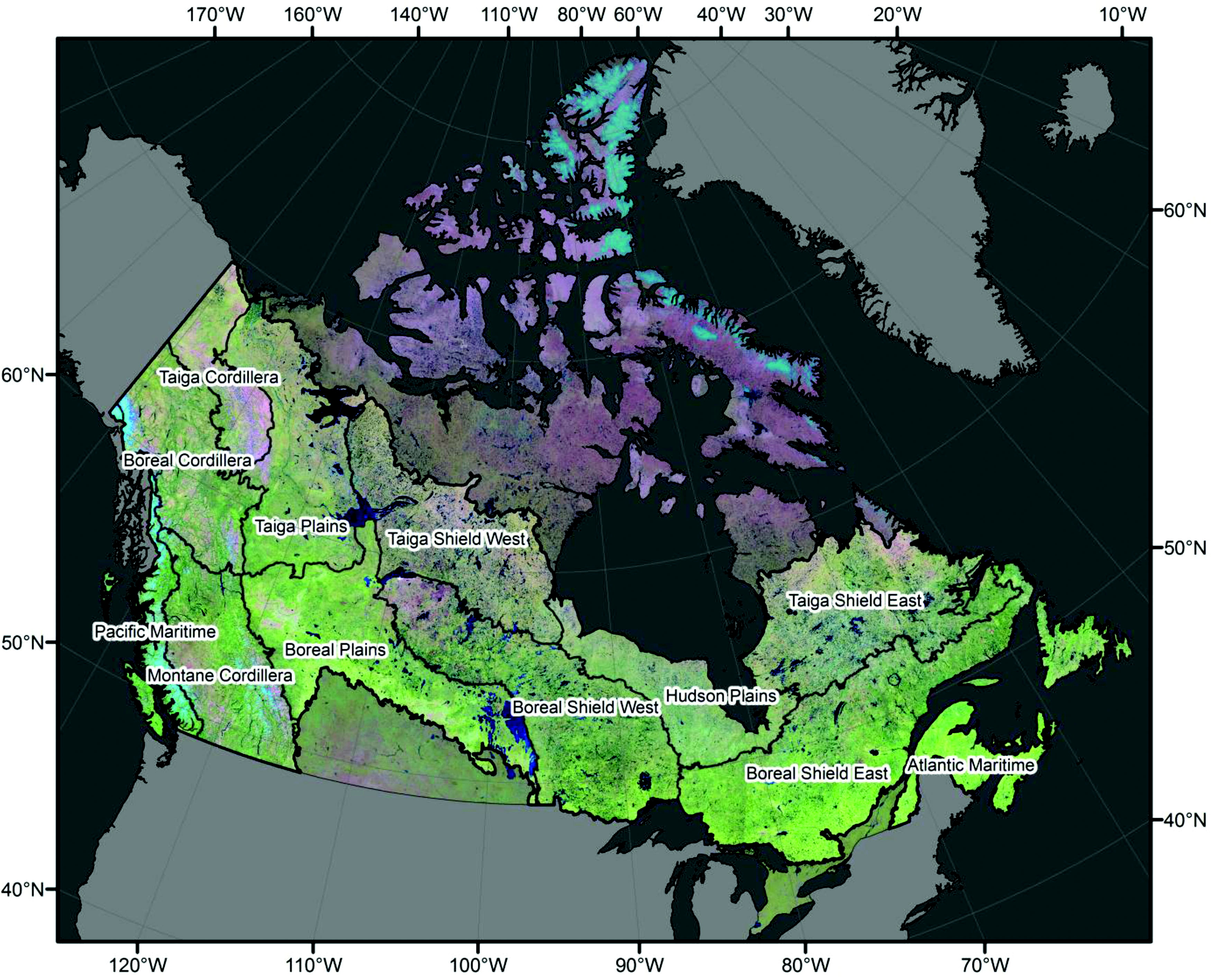
Figure 10.1: Landcover map of Canada generated by Hermosilla et al., 2018.
10.2 Types of Energy
10.2.1 Introduction
Stepping back from remote sensing for a moment, there are three general types of energy commonly used to remotely observe objects: sonic, thermal and electromagnetic. Sonic, or sound, energy is commonly used in environments where heat or light are inconsistent or hard to measure. Sonar is as example of a sonic remote sensing technique and is often deployed to observe objects in liquid. Thermal, or heat, energy is used in a variety of cases when changes in temperature indicate an underlying physiological process. An environmental example would be the observation of plant health via leaf temperature. Although both sonic and thermal energies provide useful information across a variety of disciplines, they are not the most common.
Electromagnetic radiation (EMR), which is what the human sense of sight observes, is a popular energy source in remote sensing science. At it’s most basic, this method of observation is based on the measurement of photons. Research using EMR is fundamentally interested in examining the interactions of EMR, or photons, and other particles. Before diving into the applications of EMR remote sensing (photography, spectroscopy, etc.) it is important to understand some basic theory regarding the measurement of photons.
Essentially, photons are the smallest physical property in the electromagnetic field. Photons can be emitted from objects engaged in nuclear processes (such as the sun), objects excited thermally (like a light bulb) or objects that reflect or emit absorbed radiation. The interactions between emitted photons and other particles can be observed and used to evaluate the properties of the object. A fundamental component of EMR is it’s wavelength, defined as the measured space between two consecutive peaks of a wave (IMAGE). The wavelength of a photon determines if and how it will interact with the particles around it, as well as defines the amount of energy it has. Measuring the differences in photonic energy before and after interacting with another particle is the core of any remote sensing utilizing EMR.
Perhaps the simplest path to understanding how the properties of photons (i.e. energy, wavelength) are used for remote sensing purposes is through the use of an equation. Albert Einstein explained the energy of a photon as the product of its wave frequency (the number of waves that pass a specific point over a certain amount of time) and Planck’s constant (Equation (10.1))
\[\begin{equation} E = hf \tag{10.1} \end{equation}\]Where E is the energy of a photon, h is Planck’s constant (h = 4.14 × 10⁻¹⁵ eV/s) and f is the wave frequency. Clearly, an increase in frequency results in an increase of energy. This equation may be altered to include other properties, such as the speed of light and wavelength (Equation (10.2)).
\[\begin{equation} E = hc/λ \tag{10.2} \end{equation}\]Where E is the energy of a photon, h is Planck’s constant, c is the speed of light (c = 3 x10⁸ m/s) and λ is the wavelength of the radiation. This equation contains more variables, but incorporates wavelength and in doing so utilizes an easy to measure (hc always equals 1240 eV/nm) and familiar characteristic. Due to the large range of wavelengths that photons can exhibit it is necessary to use a specific style of writing to describe them, called scientific notation.
10.2.2 Scientific Notation
Expressing extremely large or small numbers presents a challenge to both efficiency and accessibility that has existed likely since the creation of mathematics. Scientific notation presents a simple solution to this problem through simplifying numeric presentation to a value less than 10 that is raised to a particular power. Put simply, the decimal point of a large or small number is moved to make the smallest, single digit whole number. The number of places and direction that the decimal point moves is described by an associated power of 10. Equations (10.3) and (10.4) depict how large and small numbers are presented in scientific notation, respectively.
\[\begin{equation} 1,000,000 = 1.0 X 10^{6} \tag{10.3} \end{equation}\] \[\begin{equation} 0.000001 = 1.0 X 10 ^{-6} \tag{10.4} \end{equation}\]10.2.3 Electromagnetic Spectrum
Now that you have an understanding of how the properties of photons can be measured and how to write them, we can begin to explore the electromagnetic spectrum (EMS). The EMS is the continuum along within photons are located based on their properties (Figure 10.2). We have discussed both wavelength and frequency, which are inversely related and commonly used to describe EMR. Figure 10.2 also depicts a thermometer laying sideways, which demonstrates that as an object’s temperature increases, the wavelength of the photons emitted decreases. This follows Equation (10.2), which demonstrates that photons with shorter wavelengths have higher energy. A practical example of this would be that the majority of photons emitted from the sun (5,788 K) are around 0.5 x 10⁻⁶ nm, while the majority of photons emitted from the human body (~310 K) are around 10-4. These measurements are theoretical and are calculated using theoretical object, often called a blackbody that allows all energy to enter (no reflectance, hence “black”) and be absorbed (no transmission). The resulting EMR that is emitted would be generated thermally and be equal or greater than any other body at the same temperature.
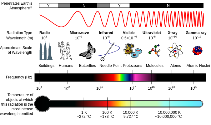
Figure 10.2: Electromagnetic (also known as Milton) spectrum depicting the type, wavelength, frequency and black body emission temperature. Credit: Inductiveload, NASA.
Call out
Visualizing the electromagnetic spectrum (EMS) in Figure 2 certainly enables a wonderful comprehension of many concepts relating to photons. Perhaps more astounding, however, is the truth of how the faculty of human vision has incorporated these properties. The portion of the EMS that humans can see is between 400 nm and 750 nm, which correlates with the most common wavelengths emitted from the sun. Perhaps it should not be surprising, but of all the possible wavelengths emitted in our environment, human eyes have evolved to maximize solar photon emission.
10.2.4 Radiation Types
Since it is possible for photon energy to vary widely across the EMS, it can be useful to group photons based on their wavelength. Generally, there are seven accepted categories. it is important to note that these categories have gradual boundaries, rather than sharp dividing lines. In order of increasing wavelength they are: radio, microwave, infrared, visible, ultraviolet, X ray and Gamma ray. We will detail each of these seven groups in Table 1 (Zwinkels 2015). If you wish a visual tour of the EMS you can explore this document created by Ginger Butcher for NASA in 2010.
| Name | Wavelength |
|---|---|
| Radio | 1 cm - 1,000 km (103 - 1010) |
| Microwave | 1 mm - 1 cm (1010 - 1011) |
| Infrared (IR) | 700 nm - 1 mm (1011 - 1014) |
| Visible (Vis) | 400 - 700 nm (1014 - 1015) |
| Ultraviolet (UV) | 10 - 400 nm (1015 - 1017) |
| X rays | 0.1 - 10 nm (1017 - 1020) |
| Gamma rays | < 0.1 nm (1020 - 1023) |
10.3 Physical laws of radiation
With a solid grasp of why EMR is useful for remote sensing science and how EMR is categorized along the EMS, we can begin to apply this core knowledge with ideas and applications related to practical use. As with radiation, there are a plethora of terms used to describe the fundamental concepts that make remote sensing science possible. Some of the most common terms have been included below. They are organized into three categories: Radiation Basics, Foundations of Measurement and Methods of Normalization.
Radiation Basics
The use of radiation to quantify properties of an object is inherently linked with relatively complex theories of physics. To minimize both confusion and workload, we will highlight a select number of key concepts that support the use of the EMS for remote sensing. The first concepts to become familiar with are radiant energy and radiant flux
Radiant energy is essentially the energy carried by photons, which is measured in Joules (J). Recall that the amount photon energy defines what wavelength (Equation (10.2). Radiant flux, which is interchangeable with radiant power, is the amount of radiant energy that is emitted, reflected, transmitted or absorbed by an object per unit time. Radiant flux considers energy at all wavelengths and is often measured per second, making it’s SI Watts (W), which is simply Joules per second (J/s) . Spectral flux is an associate of radiant flux and simply reports the amount of energy per wavelength (W/nm) or (W/Hz). Combined, these two terms allow us to describe the interaction with electromagnetic radiation and it’s environment; radiant energy interacts with an object, which results in radiant flux.
Now that you are familiar radiant energy and flux, we can discuss irradiance. Irradiance refers to the amount of radiant energy that contacts a 1 m-2 area each second (W.m-2). This includes all electromagnetic energy that contacts our 1 m-2 surface, which could be a combination of radiation from the sun, a halogen light bulb overhead and your computer screen. Another important concept is solar irradiance, which strictly refers to the amount of solar radiation interacting with our 1 m-2 area. Solar irradiance is very important in many remote sensing applications as it determines which photons an optical sensor could record in naturally illuminated environments. An associate of irradiance is radiance, which refers the the amount of radiant flux is a specific direction. The direction in question is often called the “solid angle” and makes radiance a directional quantity. You could imagine holding a DLSR camera 90 degrees above a flat leaf so that the only item visible to the shutter is the leaf. The camera would capture the radiance reflected from the leafs surface and the solid angle would be 90 degrees. Essentially, irradiance is used to measure the radiant energy that contacts a 1 m-2 area, while radiance measures the radiant flux of an object from a specific angle.
So far we have discussed radiant energy and flux as basic concepts interacting with a single object (leaf) or 1 m-2 surface. In reality, radiant energy from the sun begins interacting with objects as soon as it enters earth’s atmosphere. The process by which radiation is reflected by other particles is called scattering. Scattering occurs throughout the atmosphere and is generally separated into three categories: Rayleigh, Mie and Non-selective.
The three categories of atmospheric scattering are defined by the energy’s wavelength and the size of the interacting particle. When the wavelength of incoming radiation is larger than the particles (gases and water vapor) with which it interacts, Rayleigh scattering occurs. Phenomenon related to Rayleigh scattering include Earth’s sky appearing blue. When the wavelength of incoming radiation is similar to that of the particles with which it interacts Mie scattering occurs. The size of particles generally considered to similar is between 0.1 - 10 times that of the wavelength. Smoke and dust are common causes of Mie scattering. A third type of scattering occurs when the particles involved are lager than the wavelength of the incoming radiation. This is called non-selective scattering and results in the uniform scattering of light regardless of the wavelength. Examples of non-selective scattering are clouds and fog.
The combination of these three scattering types leads to drastic differences between the amount of solar irradiance at the top of the atmosphere and at sea level (Figure 10.3). There are also a variety of wavelengths at which ozone, oxygen, water and carbon dioxide absorb incoming radiation, precluding entire sections of the EMS from reaching the surface. Overall, only a small portion of energy emitted from the sun reaches the Earth’s surface. Most energy is absorbed or scattered by particles in the Earth’s atmosphere
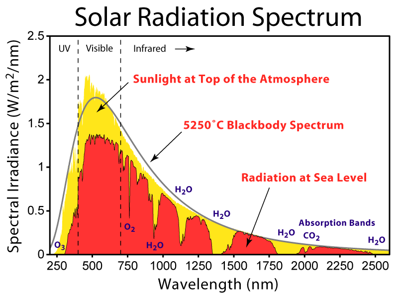
Figure 10.3: Solar radiation spectrum from 250 - 2500 nm. Irradiance measurements at the top of the atmosphere (yellow) and sea level (red) are depicted. The grey line represents the theoretical curve of a 5250 degree C blackbody spectrum. Created by Robert A. Rohde for Global Warming Arts (CC BY-SA 3.0), 2007.
The process of scattering is also affected by the properties with which it interacts. The angle at which EMR interacts with a surface, as well as the surface material, determine the properties of reflection. A reflector is described based on the properties of EMR that are reflected from it and range from specular to diffuse. Specular reflectance occurs when EMR is reflected in a single direction and can also be called ansiotropic reflectance. A mirror is an example of a specular reflector. A diffuse, or Lambertian, reflector reflects EMR in all directions equally and can also be called an isotropic reflector. An example of a surface that reflects EMR isotropically is paper.
Although specular and diffuse are measured on an spectrum four general classifications for reflectors are accepted: perfect specular, near-perfect specular, near-perfect diffuse and perfect diffuse. diffuse surfaces tend to be the most useful for remote sensing as they scatter light in all directions. This is useful because sensors can only view a surface from a single angle and can also be moving. Attempting to determine the angle at which EMR is reflected would make many projects unfeasible, especially those covering large areas.
This is not to say that diffuse reflectors are perfect, however, as some issues remain related to the angle of incidence and the position of the sensor. For example, both back scattering and forward scattering affect the amount of radiation that reaches a sensor, depending on where the sensor is located. If a sensor is observing an object at the same angle as the incident radiation, the majority of reflected EMR will be from backscatter, or EMR that is scattered back towards its source. If the object being observed is perfectly specular, no EMR reflected off the object would be captured by the sensor. If the object is a diffuse or near-perfect diffuse reflector, then there is less of a concern with regards to capturing reflected EMR.
Foundations of Measurement
Now that we have discussed radiant energy and the concepts underpinning its interactions with other objects, we can begin to explore the measurements that our sensors record. One of the most important concepts to understand is that of the spectral signature, or spectra. A spectral signature refers to the amount of electromagnetic energy recorded across a defined section of the EMS. A nice example of a spectral signature is Figure 10.3, which presents the sun’s radiation between 250 - 2500 nm in the units of solar irradiance (W/m-2/nm). Similar graphs are common throughout remote sensing and can employ different units of measure.
The base measurements taken to generate spectral signatures is of an objects radiance. Acquiring radiance across a defined section of the EMS can be conducted by a variety of sensors and at different spatial scales, highlighting the practical advantages of evaluating surfaces using EMR. To fully capture and compare the objects being measured, however, it is often necessary to normalize radiance. The need for normalization stems mainly from the aforementioned issues of atmospheric effects, source and sensor location and sensor calibration. As with any normalization, the first step is to identify our minimum and maximum values.
There are two common reference measurements used to determine minimum and maximum radiance: dark and white reference. A dark reference is often taken by measuring the amount of energy recorded by a sensor when the input device is ignored. In theory, this would be the internal darkness of the machine and is considered to be the minimum radiance value in practice. The maximum radiance value is slight more challenging to determine as it requires a perfectly diffuse, flat white surface. A commonly used material is Spectralon, which has almost 100% reflectance between 400 - 1500 nm and greater than 95% reflectance over the entire optical region of the EMS (250 - 2500 nm). With both minimum and maximum values defined, it becomes possible to calculate normalized spectral values for a variety of properties across changing conditions.
Methods of Normalization
Upon calibrating an instrument to both 100% and 0% reflectance, it is possible to determine three normalized measurements of EMR: reflectance, transmittance and absorption. Each of these measurements provides useful information for understanding the interactions between EMR and the environment.
Reflectance refers EMR that has interacted with and effectively bounced back. It has emerged as a popular method of evaluating a variety of environmental properties, including land use change, plant health and plant diversity (Asner et al. 2011). Another popular normalized measure of the interaction between photons and a surface is transmittance. A photon that is transmitted has passed through the surface with which it interacted and provides insight regarding how much energy can reach other surfaces below. In a forestry context, this information can be particularly useful when determining the amount of radiation that reaches below the upper canopy (cite LAI, etc.). Absorptance is a third, related measurement that refers to the amount of energy absorbed by the cells within a surface and is roughly equal to the amount of energy not captured as reflectance or transmittance (Equation (10.5)).
\[\begin{equation} Absorptance = 1 - Reflectance - Transmittance \tag{10.5} \end{equation}\]Although relatively straight forward, these definitions allow us to start exploring a variety of remote sensing applications. In fact, most optical remote sensing techniques employ at least one of reflectance, transmittance and absorptance to examine the world. Before moving on to the next section, please review the work flow below highlighting what we have learned so far. In our next steps we will move from theory to application and begin to explore the factors that define the quality, and therefore capability, of remotely sensed data.
Your turn!
Calculate:
The number of zeros in 2.5 x 10⁻⁷
The energy (E) of a photon with a wavelength of 450 nm.
The absorptance value for a surface with a reflectance of 0.4 and a transmittance of 0.35
10.4 The Four Resolutions
One of the first considerations any user must make regarding remotely sensed data is its quality. For most scientific research, good quality data needs to contain information that is relevant to the scale and time period of the study. It would be challenging, for example, to evaluate the changes in vegetation cover in Vancouver, B.C. from 2010 - 2020 by looking at a single image of Calgary, Alberta from 1995. Although this example may seem extreme, it highlights the need for data collectors and users to communicate about where, when and what is included in a dataset. Enter the Four Resolutions.
10.4.1 Spatial Resolution
Although each resolution is important, spatial resolution holds a key position when determine the usefulness of a dataset as it determines the scale at which information is collected. When a sensor collects information it does so in a single area. That area could be the size of a single tree or a single city, but all the EMR measured by the sensor will be an average of that area. Generally, this area is referred to as a picture element, or pixel. A pixel is the smallest addressable digital element and basic unit of remotely sensed data. When multiple pixels are collected in adjacent areas, perhaps using an instrument with multiple sensors on it, the output is called an image. In short, an image is a collection of pixels, which represent mean values of the area they represent. Spatial resolution, then, is the ground area represented by a pixel.
There are a variety of factors that affect spatial resolution, or the size of a pixel. One important factor is the sensor’s field of view (FOV). A field of view refers to the observable area of a sensor and is defined by two things: the angle of the FOV and the sensors distance from it’s target. Changes in these two factors result in an increase or decrease in the amount of area captured by a senor and therefore a change in pixel size. Pixels that cover larger areas are considered to have lower spatial resolution, while a relatively smaller pixel is considered high resolution. When a sensor is in motion, collecting multiple pixels across space and time, the term instantaneous field of view (IFOV) is used to describe the FOV at the time each pixel was collected. We will learn more about the challenges of collecting data over space and time in Chapters 12 and 15.
To determine if a certain spatial resolution is useful, then it would need to be detailed enough to include the features of interest, but large enough to be stored and processed in a reasonable manner. It must also cover the entire study area, which can vary significantly depending on the research objectives. Each of these considerations will direct the data user to a specific sensor. From here, the user can begin to consider the remaining three resolutions.
10.4.2 Temporal Resolution
Much like spatial resolutions deals with the space that a sensor observes, temporal resolution refers to the time interval between successive observations of a given space. Temporal resolution can span seconds or years and is requirement when investigating change. Much like spatial resolution, an acceptable temporal resolution is defined inherently by the nature of the study. For example, a study monitoring the annual urban expansion of Vancouver, B.C. would have a temporal resolution of 1 year.
10.4.3 Spectral Resolution
Earlier in this chapter the concepts and theories surrounding EMR were presented. These theories related directly to the concept of spectral resolution, which refers to the number and dimension of specific EMR wavelengths that a remote sensing instrument can measure. Due to the large range of the EMS and properties of EMR, the term spectral resolution is often used to refer to any single component of its definition. In scientific literature, it is not uncommon to find “spectral resolution” referring to:
the number of spectral bands (discrete regions of the EMS) that are sensed as a single unit.
the location of these units, or groups of bands, along the EMS.
the number of individual bands within each unit. Also called bandwidth.
Each of these components plays a role is describing the spectral resolution of a pixel and enables users to identify appropriate sensors for their application. It is also important to consider the laws associated with the energy of EMR. Recall that shorter wavelengths have more energy, which makes it easier to detect. The implications of this is that longer wavelengths require larger bandwidths for the sensor to observe them. An easy visualization of this concept involves selecting two wavelengths along the EMS. If we select the first wavelength at 0.4 and the second wavelength at 0.8, we can use Equation (10.2) to demonstrate that the first wavelength has twice as much energy as the second. This is an important theory to note as the consequences of a decrease in energy is a decrease in spatial resolution (a larger number of bands need to be combined to collect enough information).
A common method for visualizing the spectral resolution of a sensor is to place each band along the EMS according to it’s associated bandwidth and wavelengths (Figure 10.4). This allows users to determine which sensor best captures the information they are interested in studying. For some applications, such as land use, it is acceptable to use sensors with relatively wide bands collecting information in a small number of strategic locations along the EMS. For other applications, spectral information may need to be more detailed and capture information using thin, adjacent bands spanning a large region of the EMS. These specifications will be discussed in greater detail in Chapter 12, so for now we’ll focus on how spectral information can be useful.
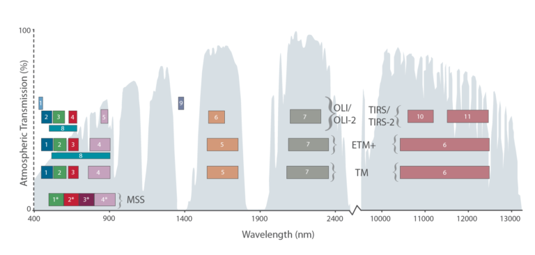
Figure 10.4: Locations of bands for various sensors deployed by NASA on one of more Landsat misison. Landsat 1-5 had the Multispectral Scanner System (MSS), while the Thematic Mapper (TM) was aboard Landsat 4-5. The Enrinched TM Plus (ETM+) had 8 bands and was aboard Landsat 7. Grey distributions in the background represent the atmospheric transmission values for a mid-latitude, hazy, summer atmosphere. This image was created by NASA.
The collection of spectral data across more than one band allows the creation of a spectral curve, or spectral signature. Spectral signature are the cornerstone of many remote sensing applications and highlight many properties of the surface from which they were collected. The creation of a spectral signature is quite simple and can be depicted in two dimensions (Figure 10.5. Essentially, the observed value of each band is connected to the observed value of each adjacent band in 2D space. When all bands are connected, a spectral signature is born. As we will see in a later case study, spectral signatures can provide a plethora of relevant information relating to the composition of an object.
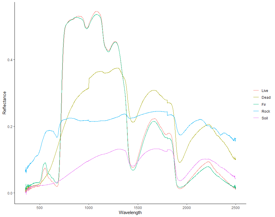
Figure 10.5: Five spectral signatures of various living and non-living samples collected using an ASD FieldSpec3 Imaging Spectroradiometer.
10.4.4 Radiometric Resolution
In short, radiometric resolution is the quantifaction of a sensors ability to detect differences in energy. Photons enter a sensor through a filter that only permits specific wavelengths.The energy of the photon is recorded as a digital number (DN) and the digital number is assigned to a pixel.
A simple visualization of radiometric resolution would be to think of three colors: red, green and blue (Figure Cambridge in color). A sensor detecting energy in the ranges of these three wavelengths would contain three separate detectors. Each detector is specialized to record energy in a single, unique range, say red (~700 nm). The amount of energy that is recorded while observing an area is stored in a pixel as a DN, with the lowest DN number representing zero energy in this wavelength range and the highest DN representing maximum energy.
The radiometric resolution of a detector, then, is the number of segments present between zero and maximum DN values. These segments are usually referred to as bits and can be mathematically represented as an exponent of 2 (Equation (10.6)). The number of bits in that a detector can resolve may also be called the color depth of the image. Figure clearly presents the increase in detail provided by additional bits, but recall that increasing any resolution generally increases storage and processing time. As such, it is important to select an appropriate radiometric resolution based on the needs of your study.
\[\begin{equation} 8 bits = 2^8 = 256 levels \tag{10.6} \end{equation}\]10.5 Key Applications
So far in this chapter we have covered the theories and concepts that justify the use of EMR for remote sensing. With these fundamentals in mind, we can begin discussing some common applications of remote sensing. For the purposes of this book, we will focus on studies related to environmental management.
The use of optical remote sensing (400 - 2500 nm) to analyze the environment has become popular over the past half century. Sensor development, improved deployability and decreasing costs have enabled many researchers to use selected sections of the EMS to monitor everything from the chlorophyll content of a single leaf (Curran 1989) to global forest cover (Hansen et al. 2013).
Large-scale research projects focused at national or international levels have perhaps benefit the most from improved sensor deployment. Since 1972, a variety of satellites have been launched with the sole purpose of observing the Earth. Landsat is NASA suite of satellites designed specifically for this purpose. By the end of 2021, a total of nine Landsat missions will have been launched, eight of which have successfully reached orbit and provided imagery in at least 5 broad spectral bands at 30 m-2 spatial resolution. This information has been used to monitor of land cover change, ecosystem services and a variety of other environmentally relevant metrics (Deel et al. 2012). The case study at the end of this section highlights a particularly novel approach to optical remote sensing that has become a popular methodology to evaluate plant health and biodiversity (Ustin et al. 2009)(Wang et al. 2018).
As far as Canada’s contributions to remote sensing sensors rank, RADARsat is among the most important (Raney et al. 1991). This satellite was launched in 1995 and has grown to a constellation of three space-borne synthetic aperture radar (SAR) sensors that feature variable resolution. As an active sensor, RADARsat produces and measures EMR with wavelengths between 7.5 - 15 cm and is capable of penetrating clouds and smoke (Raney et al. 1991). It’s active nature also enables RADARsat to record observations at night. Chapter 12 will discuss radar in more detail.
Another active remote sensing technique that has become popular is light detection and ranging (LiDAR), which can also be called airborne laser scanning (ALS). LiDAR is particularly useful in evaluating structural components of the environment, such as forest canopies and elevation (Coops et al. 2007). More details regarding the theories and applications of LIDAR will be presented in Chapter 15.
Case Study
Optical remote sensing detects functional and biological diversity in South American ecosystems
In 2009 Asner and Martin presented the concept of airborne spectranomics Asner and Martin (2009). Their idea was based on the fact that plant leaf tissues contain a variety of different components that are associated with underlying environmental conditions and that variations in these components can be captured by observing their effects on electromagnetic radiation (Figure 10.6). They proposed a method that linked leaf functional traits, both structural and chemical, to leaf reflectance between 400 - 2500 nm using partial least squares regression (PLSR) modeling. They demonstrated that these models could accurately predict the leaf traits in questions and proved that this methodology could be scaled to the canopy-level. Asner and Martin also showed that plant species could be accurately grouped based on the similarities of their spectral signatures (Figure 10.7). Combined, these concepts enabled the accurate detection of functional and biological diversity across both the Andes and Amazon region of South America.
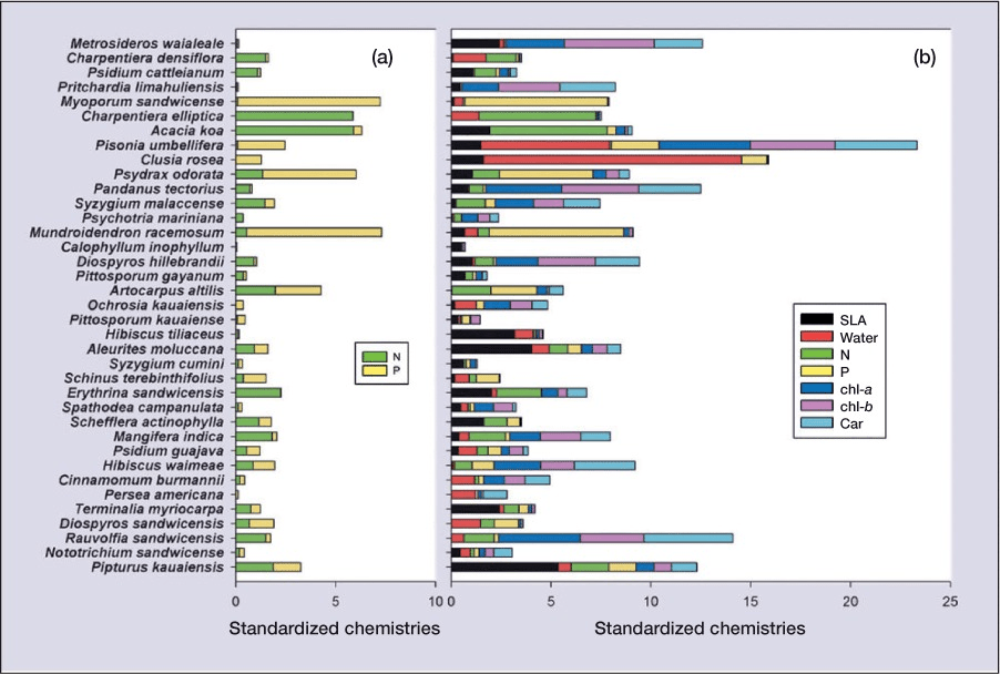
Figure 10.6: Funcitonal traits of canopy species presented in Asner and Martin 2009 presented. The comparison of (a) leaf nitrogen (N) and phosphorous (P) with (b) an enhanced trait array of seven traits (chl-a and -b = chlorophyll-a and -b, respectively, SLA = specific leaf area, Car = carotenoids) highlights the increased capacity for differentiation generated through the consideration of additional traits.
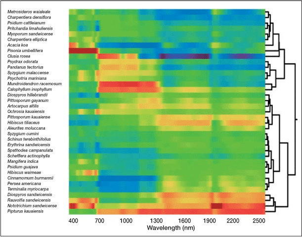
Figure 10.7: Cluster analysis of spectral signatures from 37 unique plant species conducted by Asner and Martin 2009. Red and blue represent high and low reflance values, respecively, and the dendogram presented on the right side of the graph demonstrates the assigned groupings. Figure adapted from Asner and Martin 2009.
10.6 Summary
In this chapter we have covered a variety of physical theories that support the use of electromagnetic radiation for the remote analysis of objects. Although time consuming, and perhaps not as interesting as exploring successful applications, these ideas provide the fundamental knowledge needed to employ remote sensing technologies. From sensor selection to data processing, your ability to perform remote sensing science will rely almost exclusively on your capacity to comprehend the relationships between the objects of interest and the physical properties that comprise them.
In the next chapter you will enter the world of sensors and explore a vast amount of technologies that collect information remotely. This journey will include active and passive instruments, as well as examples of scientific studies that have successfully employed the data they collect. Much like a carpenter selecting the correct tool for a specific task, you will need apply your knowledge of the fundamentals to identify the best sensor for your research.
10.6.1 Reflection Questions
- What section of the electromagnetic spectrum is adjacent to, but shorter in wavelength than, what the human eye can see?
- What is the general term used to describe the process that stops large amounts of electromagnetic radiation from reaching the Earth’s surface. Name the three types?
- List and describe the four resolutions.
- What aspect of the relationship between light and leaves did (Asner and Martin 2009) exploit to derive leaf chemicals?