Chapter 15 LiDAR Acquisition and Analysis
Bold Text, Italicized Text Regular Text.
Learning Objectives
- Understand how LiDAR works
- Understand what we can do with LiDAR data
- Understand the basic processing steps required to use LiDAR data in a forestry context
Key Terms
LiDAR, ALS, Surface Models, LiDAR Metrics, Area-Based Approach, Individual Tree Detection
15.1 What is LiDAR?
LiDAR is an active remote sensing technology that uses a laser scanner and time of flight principles to collect 3 dimensional data. A LiDAR system is made up of three components; a laser-scanning device, and accurate global navigation satellite system (GNSS), and an inertial measurement unit (IMU). The GNSS receiver allows the position of the laser to be determined in space, while the IMU records the orientation of the laser (i.e. roll, pitch, and yaw). When discussing LiDAR in an airborne context, we can also call it airborne laser scanning (ALS).
15.1.1 How does it Work?
Typical LiDAR systems use the time of flight method to produce 3D data. A laser ranging instrument produces a short, intense pulse of light from the instrument to a target being measured. Some of this energy is then reflected back to the instrument, where it is recorded. Since the speed of light, and the location of the laser ranging instrument is known, we can calculate the position of the target by timing how long it takes between the the pulse being emitted and received.
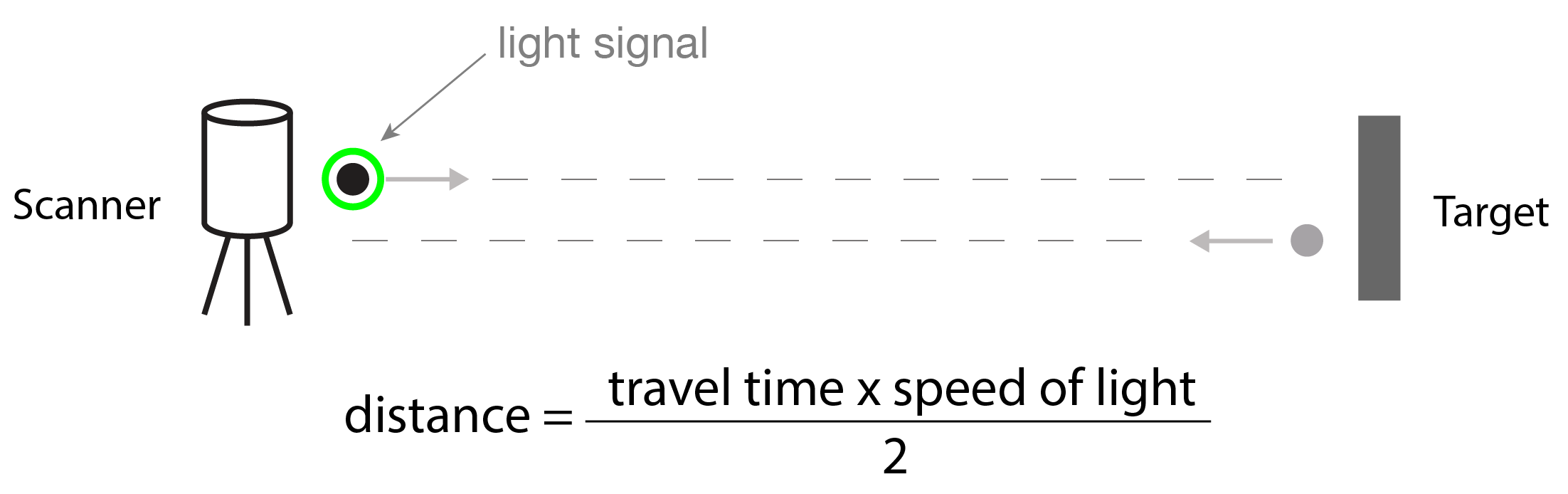
Figure X Concept of LiDAR.
A LiDAR dataset includes several pieces of information for each 3D point. X,Y,Z location data is included, as well as information about how the data was collected. In many cases, this includes
The most common file format for LiDAR files is called the LAS file format (.las). This file format was originally designed for 3-dimensional point cloud data, and is a free alternative to proprietary systems or a generic ASCII file interchange system. The main benefits of this file format are that it is relatively quick, can be used by any system, and stores information specific to the nature of LiDAR data wihtout being overly complex (:https://www.asprs.org/divisions-committees/lidar-division/laser-las-file-format-exchange-activities).
LiDAR HISTORY
Early LiDAR point densities were low, which
Brief history in forestry / what can we do with LiDAR
Figure X LiDAR System.
15.2 Components of LiDAR Systems
15.2.1 Lasers
- 4:10 - video 1
- Typical wavelengths (eye safe, NIR vs green for bathymetric)
- Power
- Beam divergence - important to take into account. Think about a dinner plate compared to a bicycle wheel. A beam that has low divergence (dinner plate) will be able to distinguish more objects than a high divergence beam (bicycle wheel).
- Target interaction - 7:45 in video 1
- Scanning types - zig-zag, rotating mirror line, push broom (call back to RS chapter?) - video 2, 2:08
- Pulse frequency, scan rate, scan angle
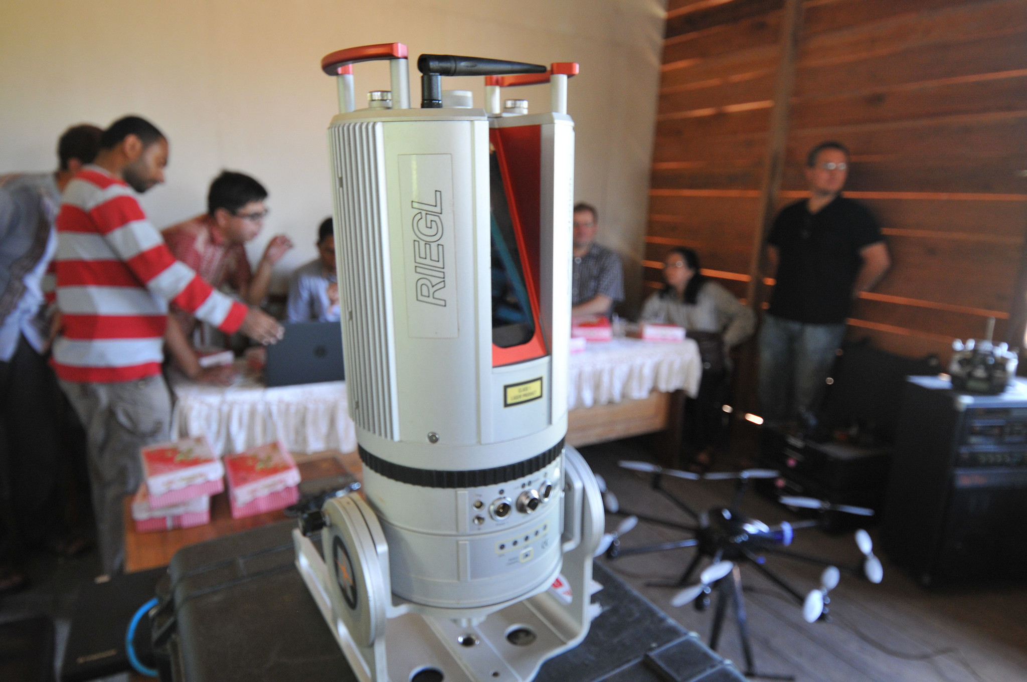
Figure X LiDAR Unit.
15.2.2 Position and Orientation
Global Navigation Satellite Systems
Require us to know our position exactly!
Callback to GNSS?
On board GPS and GPS reference stations on the ground are used to post process the data in order to be as accurate as possible
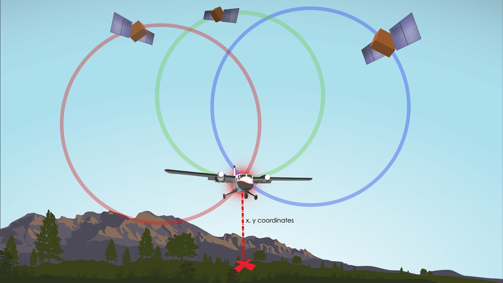
Figure X XYZ Coordinates.
Inertial Measurement Unit (IMU)
An inertial measurement unit (IMU) consists of gyroscopes and accelerometers measures the attitude and acceleration of the aircraft along the X, Y, Z axis. This data is combined with the GNSS data to provide a precise location of the scanner in space.
Mentioned elswhere? What is it - focus on image that discusses pitch/roll/yaw
Clocks
The LiDAR point data needs to be synched with the positioning data in order to know where the point is in space. To do this, a very accurate GPS clock is used to time stamp the laser scanning data (7:30 video 2).
Accurate clocks are imperative for producing accurate point clouds. One nanosecond corresponds to a 30 cm travel distance A - (video 1)
15.2.3 Platform
LiDAR units can be attached to a variety of platforms. Traditionally, LiDAR units for forestry research were mounted on airplanes and helicopters, as units were large and cumbersome [Figure X for actual scanner], however ground based units such as terrestrial laser scanning (TLS), and mobile laser scanning (MLS) have also been developed. These units tend to have a very high point density, and TLS is often used in modeling tree architecture.
Plane vs helicopter - what is normal
Drone: As technology has improved and laser units have gotten smaller, we can mount LiDAR units to drones (also known as…)
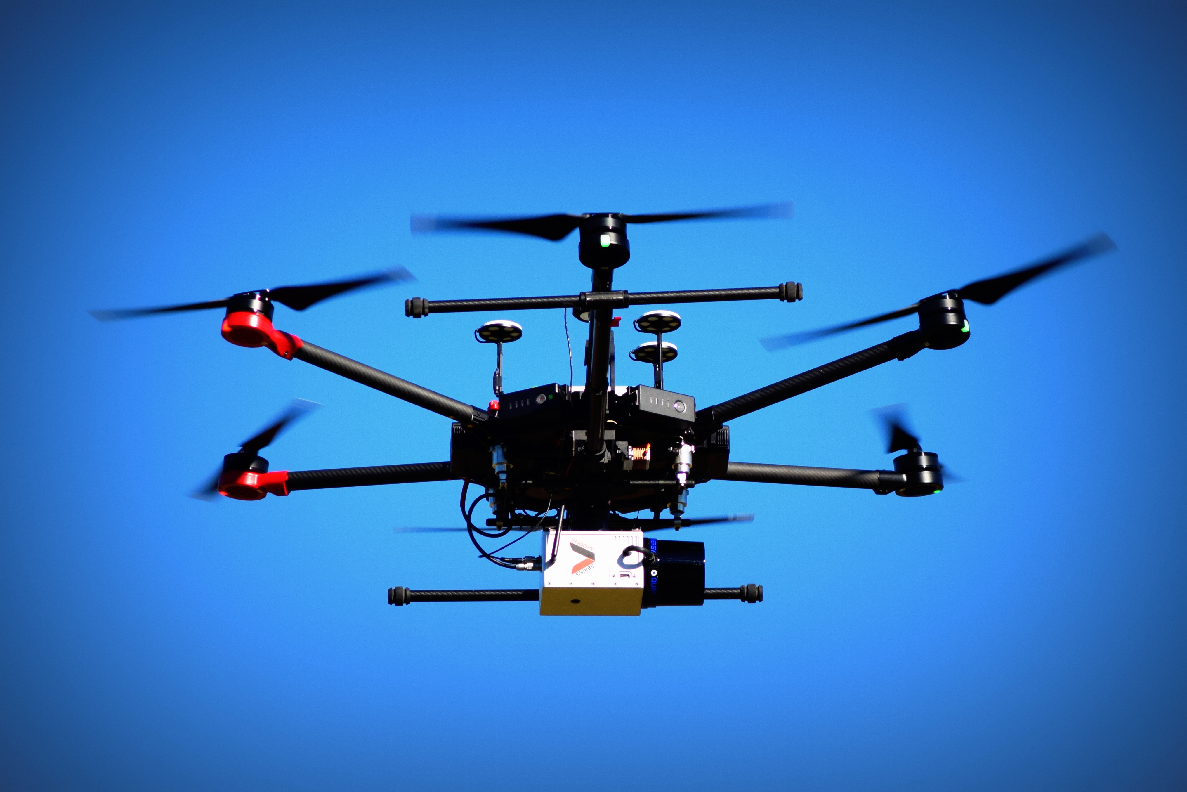
Figure X Drone mounted LiDAR.
MLS/backpack
Satellite based:
ICESat
GEDI
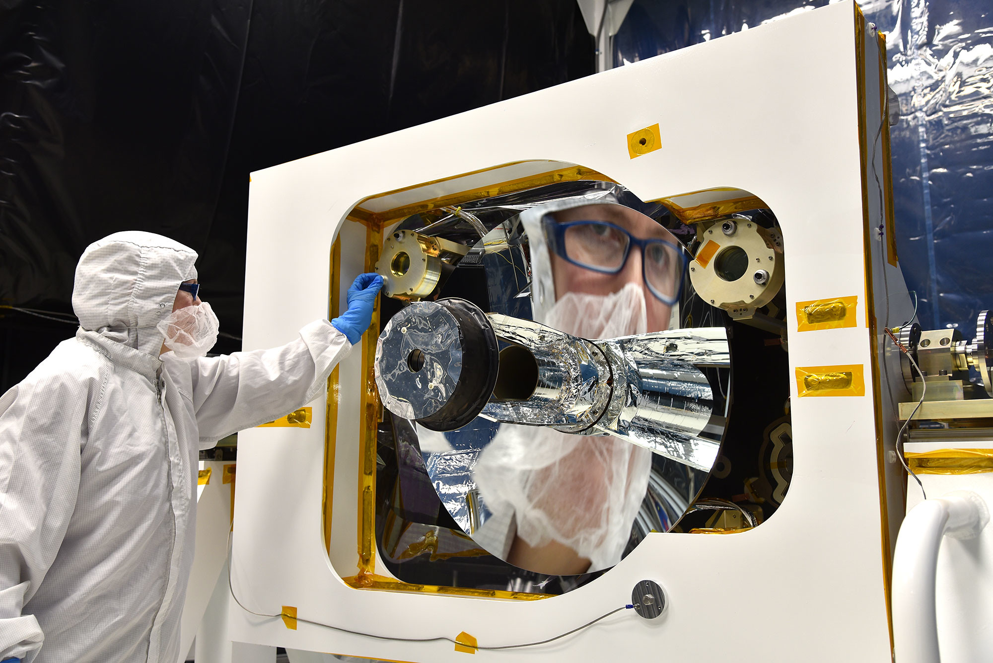
Figure X GEDI.
- Cars: Don’t need figure..
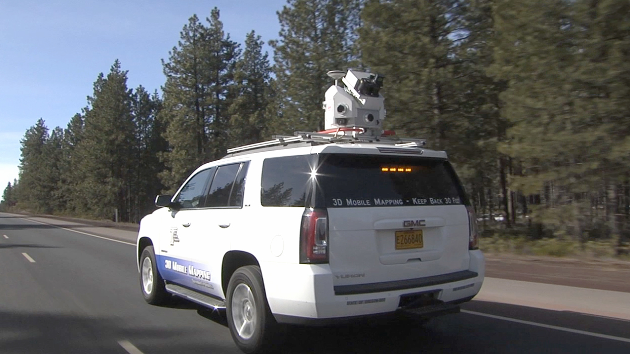
Figure X Mobile LiDAR System.
- TLS
IDEA: combine different types into one collage
15.3 Types of LiDAR
15.3.1 Discrete Return
Discrete return LiDAR = more common. Include figure of a cross-section!
15.3.2 Full Waveform
15.3.3 Multispectral
- New
15.3.4 Single Photon Lidar
- New
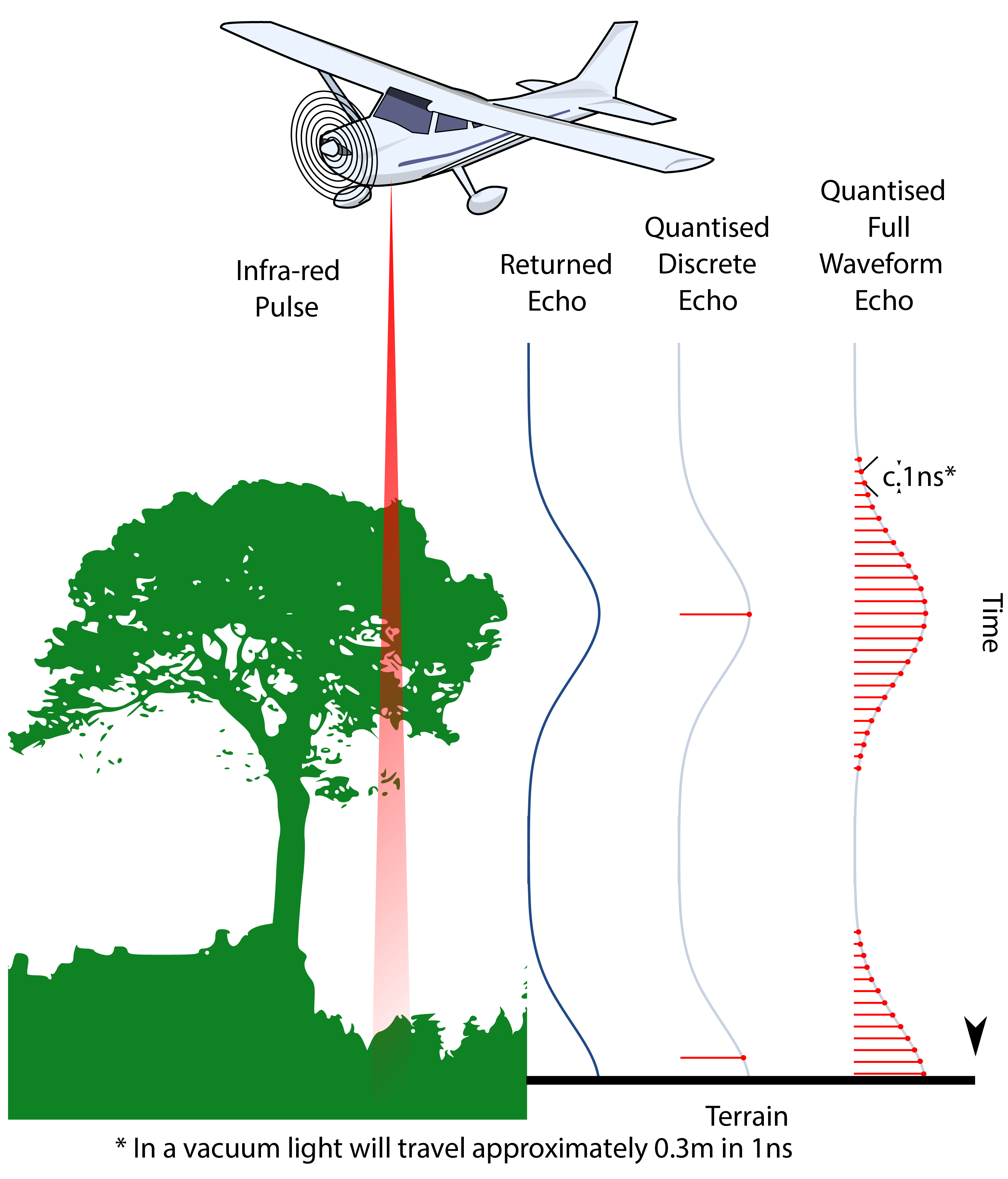
Figure X LiDAR Discrete vs Full Waveform.
Lorem ipsum dolor sit amet, consectetur adipiscing elit. Ut in dolor nibh. Lorem ipsum dolor sit amet, consectetur adipiscing elit.
Call out
This is a call out. Put some important concept or fact in here.
15.4 LiDAR Derivatives and Analysis
- What can we do with LiDAR derivatives, why are they important
- What is the use for LiDAR in forestry and ecology - examples from NCC LiDAR Lecture
- How do we go from raw cloud to these derivatives
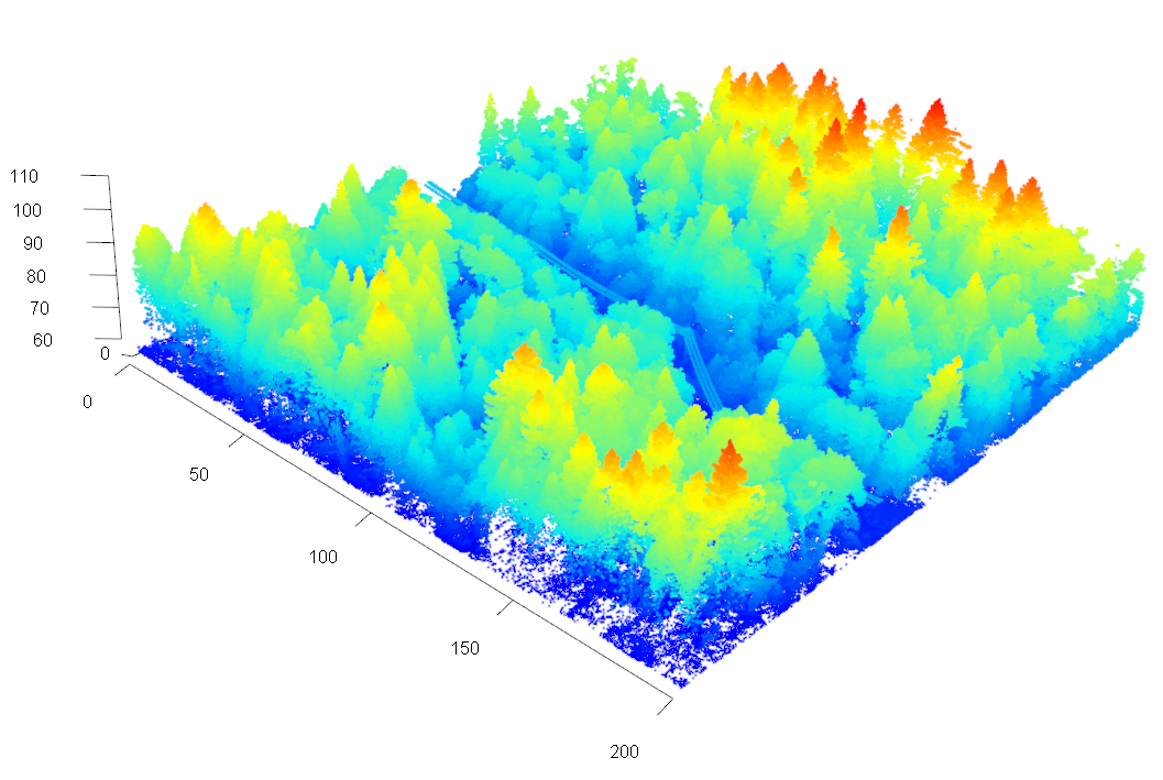
Figure X typical LiDAR point cloud.
15.4.1 Bare Earth Elevation
- What is a DEM
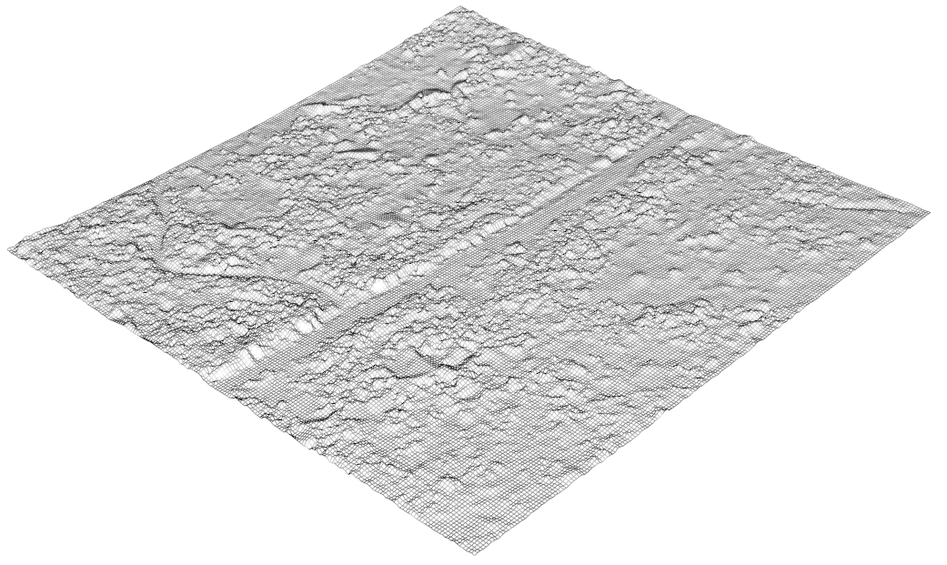
Figure X DEM.
15.4.2 Canopy Height Model
- What is a CHM
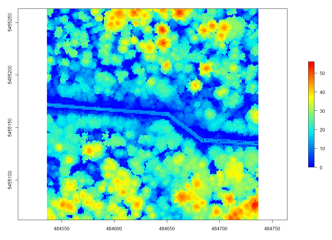
Figure X CHM.
15.4.3 Canopy Surface Model
- CHM vs DSM?
15.4.4 Grid Metrics
- What are these used for
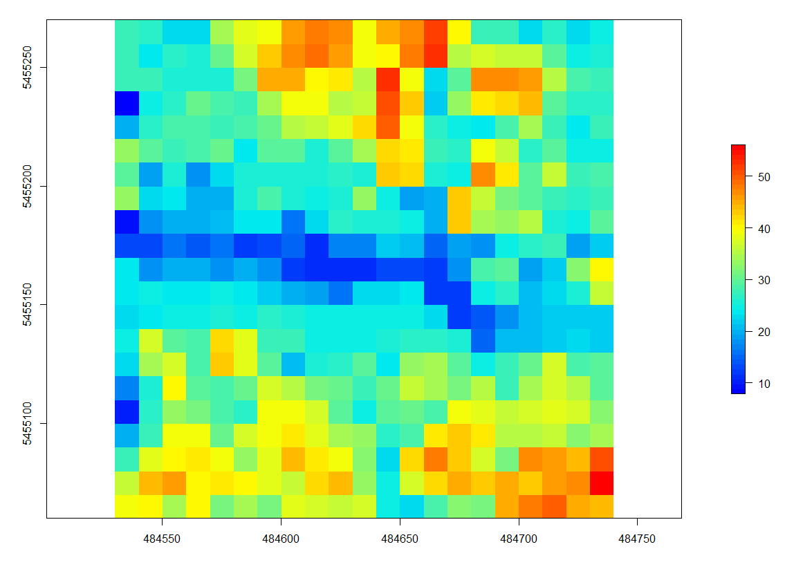
Figure X DEM.
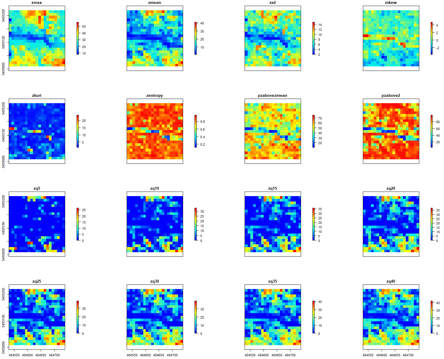
Figure X DEM.
15.4.5 Tree Segmentation
-How and why would we want too do this
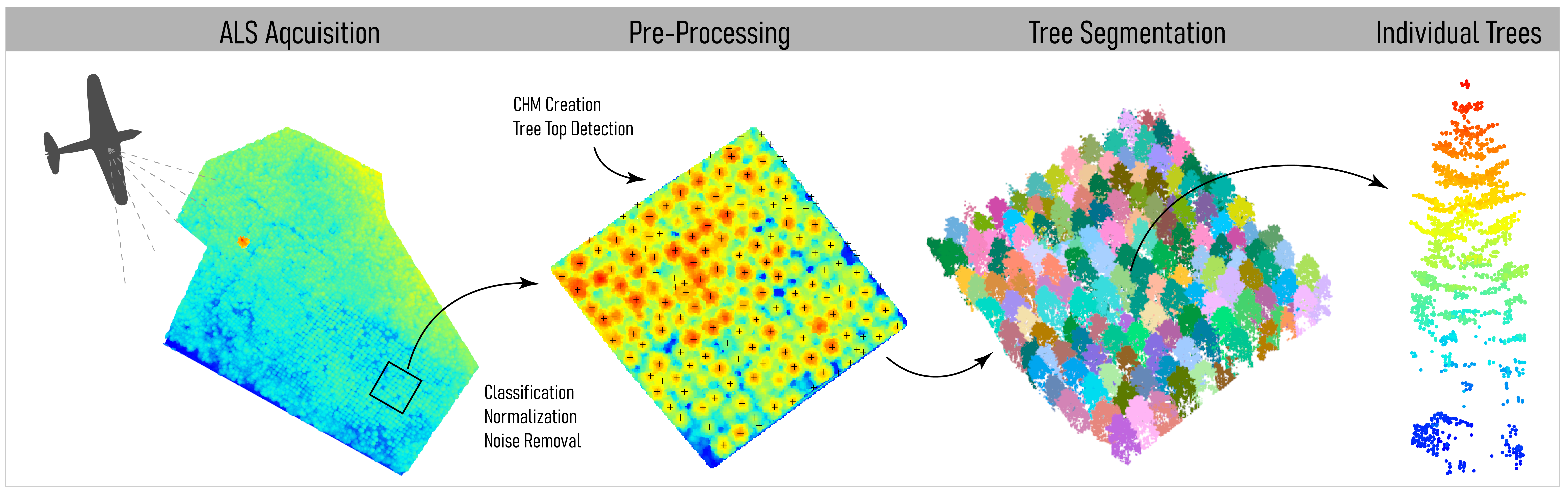
Figure X Processing Flowchart.
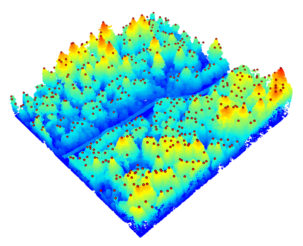
Figure X DEM.
15.4.6 Software
We use lidR for this section.. Can use XYZ
Case Study
Creating LiDAR Metrics from a Raw Point Cloud
For this case study, we will be using a clipped .las file from the 2018 open LiDAR dataset of City of Vancouver and UBC Endowment Lands in British Columbia (we randomly selected a 200 x 200 meter portion of the ‘4840E_54550N’ tile, see below for the link where you can download the data), and the lidR package in R. The script to process this data is included HERE [where to include script?], and you can use the lidR book [link] to get a more in depth understanding of the functions we apply below.
The first step when looking at LiDAR data is to inspect it; we recommend using the free software CloudCompare (link below), or the plot() function in the lidR package. Once we have a sense of our data, we can clean and filter the data, using classify_noise() and the ‘-drop’ switch to get rid of the noise in our dataset [include image showing noisy vs. clean data?]. Our cleaned dataset can then be used to create a DEM; first we can classify_ground(), followed by using the grid_terrain() function [call back to previous chapter] – this is an essential step that could require quite a bit of tweaking depending on what you want to use the DEM for! In our case, the DEM is used to normalize the point cloud. Normalization removes the effect of terrain on above ground measurements, allowing comparisons of vegetation heights. [insert image of DEM and CHM]. The normalized point cloud is used to create our CHM (created using grid_canopy()). It is at this point that we can analyze the point cloud in a variety of ways. We can use an area-based approach (ABA) to create metrics at the grid level (grid_metrics()), or we can derive metrics at the individual tree scale. In order to do this we need to first segment the trees (segment_trees()) before creating metrics (tree_metrics()). Below we can see an example of a segmented point cloud.
Case studies should have at least one image or map (no more than 2 total) and the written length should be around 300 words (shown above). Any references to external literature should by hyperlinked with the Digitial Object Identifier (DOI) permanent URL and entered into the bibliography. Avoid linking to external resources without a DOI and permanent URL. Contact Paul or try using the Leaflet package in R if you want to add an interactive web map.
Your turn!
Explore some of the LiDAR derivatives that we produced in the case study above
Interactive map of rasters:
DEM
CHM
and some grid metrics - e.g. mean and p99?
Screenshot vs. interactive point cloud - data size concerns
Necessity of being able to rotate point cloud? Relatively little gain for trouble of small area.
Your browser does not support iframes
15.5 Summary
LiDAR! Requires 3 components. Important for vertical characterization of the forest. Can produce useful rasters
Reflection Questions
- Explain ipsum lorem.
- Define ipsum lorem.
- What is the role of ispum lorem?
- How does ipsum lorem work?
Practice Questions
- Given ipsum, solve for lorem.
- Draw ipsum lorem.
## Recommended Readings {-}
Ensure all inline citations are properly referenced here.