Uncertainty in GIS
Uncertainty = Accuracy + Precision + Ambiguity + Vagueness + Logical Fallacies
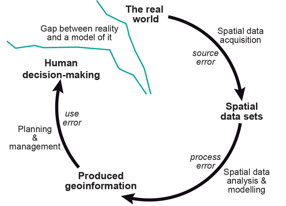
Uncertainty
Arises from our inability to measure phenomena perfectly and flaws in our conceptual models.
- Data quality: Instrument limitations, sampling costs, etc.
- Generalizations when representing phenomena: i.e., Bonini's Paradox
- Incomplete knowledge, misunderstandings, biases, etc.
Data Quality
There is no standardized measure of data quality in GIS.
- Flaws may pass through many users before discovery.
- Must trust the data was collected and processed correctly.
- Risk of the users misinterpreting valid products.

When baking mistakes are obvious.
Often in GIS, they are not.
Data Quality
Data must be assessed on a case by case basis.
- Is the resolution of the data sufficient for the scale of my analysis?
- Is this the most up to date version of this dataset?
- Can I trust the organization publishing this data?
Error: Accuracy & Precision
The terms are related, but the distinction is very important.
Accuracy: The degree to which a set of measurements correctly matches the real world values.
- How close is the measurement to the real value?
Precision: The degree of agreement between multiple measurements of the same real world phenomena.
- How repeatable is the measurement?
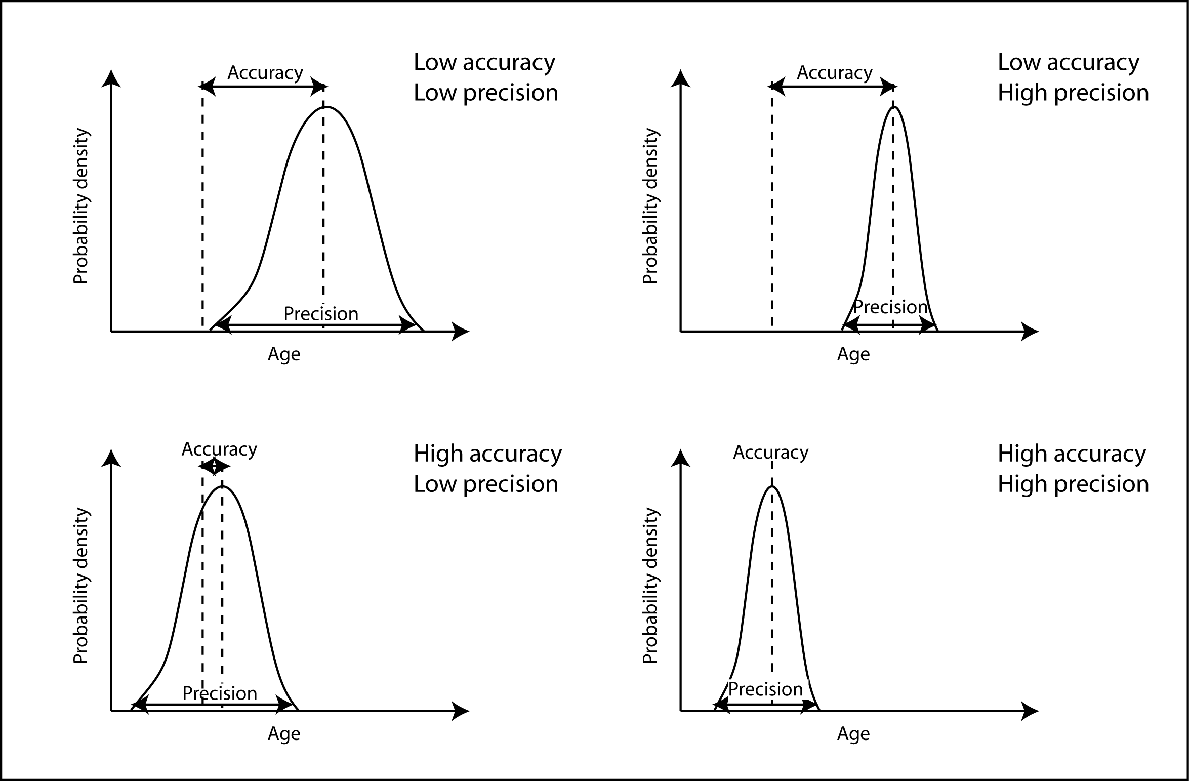
Error: Accuracy & Precision
- Accuracy: A systematic (consistent) offset from the real world value; errors have a bias.
- Precision: A random offset from the real world value; errors are unbiased
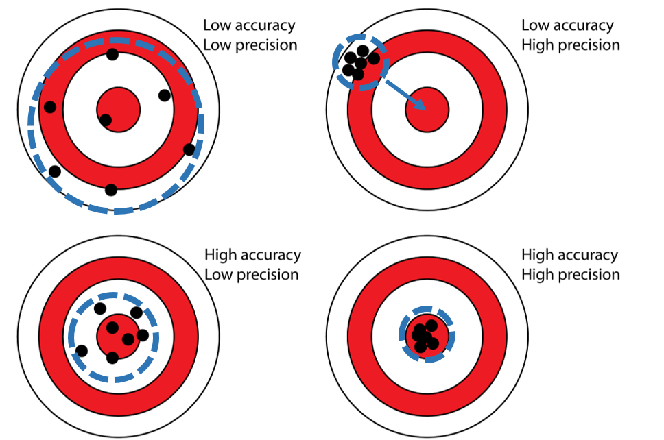
Accuracy and precision can be quantified.
Quantifying Error
Statistical methods can be used to quantify error.
- These measures won't tell us for sure that we are correct, but they can give us some insight.
We can quantify any offset (bias) and the spread of the measurements (unbiased).
Quantifying Accuracy
Mean Absolute Error (MAE):
- The absolute value of the error averaged across all samples.
- How close the samples (observations or estimate) are to be to the true values.
$MAE = \frac{\sum_{i=1}^N \lvert{x_i-t_i}\rvert}{N}$
$x_i$ = the ith sample value
$t_i$ = the ith true value
$N$ = the total number of samples
Quantifying Accuracy
Mean Squared Error (MSE):
- The squared error averaged across all samples.
- Similar to MAE, but more harshly penalizes large deviations.
- MSE is not in the same units as the original data.
$MSE = \frac{\sum_{i=1}^N \left({x_i-t_i}\right)^2}{N}$
$x_i$ = the ith sample value
$t_i$ = the ith true value
$N$ = the total number of samples
Quantifying Accuracy
Root Mean Squared Error (RMSE):
- The square root of the squared error averaged across all samples.
- Same as MSE, except:
- With the square root, RMSE is in the same units as the original data.
$RMSE = \sqrt{\frac{\sum_{i=1}^N \left({x_i-t_i}\right)^2}{N}}$
$x_i$ = the ith sample value
$t_i$ = the ith true value
$N$ = the total number of samples
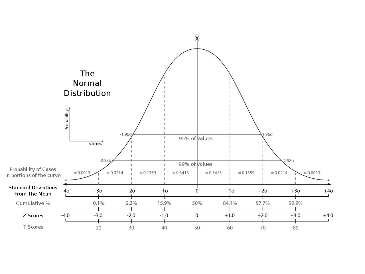
Quantifying Precision
Standard Deviation ($\sigma$):
- The square root of squared deviation averaged across all samples.
- similar to RMSE, except:
- Instead of characterizing error, it the dispersion of a dataset.
$\sigma=\sqrt{\frac{\sum_{i=1}^N \left({x_i-\overline{X}}\right)^2}{N}}$
$x_i$ = the ith sample value
$\overline{X}$ = the mean of all samples
$N$ = the total number of samples
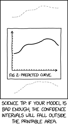
Quantifying Precision
Confidence Intervals (CI):
- Used to convey our confidence in the estimated average value.
- If the $x$ values are close together, we have higher confidence in $\overline{X}$.
- If the $x$ values are more dispersed, we have lower confidence in $\overline{X}$.
$CI = \frac{\sigma}{\sqrt{N}} z$
$\sigma$ = the standard deviation
$N$ = the total number of samples
$z$ = a z-score
Quantifying Precision
Confidence Intervals (CI):
- For Normally Distributed data:
- Can be used to specify a confidence level (i.e., 90%, 95%, etc).
- Typically presented as a range around the mean.
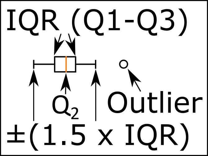
Quantifying Precision
Inter Quartile Range (IQR):
- For Non-normally Distributed data:
- Cannot be used to specify a confidence level.
- But it can give us some idea of the dispersion in a dataset.
Vagueness and Ambiguity
The terms are related, but the distinction is very important.
Vagueness: When something is not clearly stated or defined.
- Arises when boundaries or labels are poorly defined.
Ambiguity: When something can reasonably be interpreted in multiple ways.
- Arises when terms or labels can apply to multiple features.
Vagueness
- What does “London” refer to:
- London, UK?
- London, Ontario?
- London Drugs?
- The word "bank":
- A financial institution?
- The edge of a river?
Ambiguity
- Interpretation requires context.
- Where does a forest end and a grassland begin?
- The position of objects are unclear or changeable.
- Coastal boundary file - High tide? Low tide? Mean water level?

Qualifying Vagueness and Ambiguity
Ambiguity and vagueness are difficult to quantify numerically. But they still must be addressed whenever possible..
The key with these issues:
- Present things clearly and thoroughly. Be explicit and transparent when conducting and communicating your work.
Sources of Uncertainty
Where does uncertainty come from and what can we do to minimize it?
Measurements
Some sources of error are out of our control. The instruments we use to collect data can only so precise.
- It is actually impossible to know all the physical quantities of an object.
- Heisenberg Uncertainty Principle: you cannot concurrently measure a particles exact position and momentum!
Data Resolution
The concentration of samples in space and time dictates the level of accuracy & precision you can attain.
- Lower resolution data is by definition less precise, but not necessarily less accurate.
- High resolution data can be very precise, but have a significant bias.
- What do you do if your data are collected at different resolutions?
- Low resolution result in vagueness & ambiguity.
Data Entry
Things we do have some control over:
- Input datasets & sample sizes.
- Typos during tabular data entry.
- Digitizing errors when creating vector features.
- Gaps: there should be a feature, but there is not.
- Overlaps: one polygon sits over another polygon.
- Slivers: a feature is created between two features when it should not be.
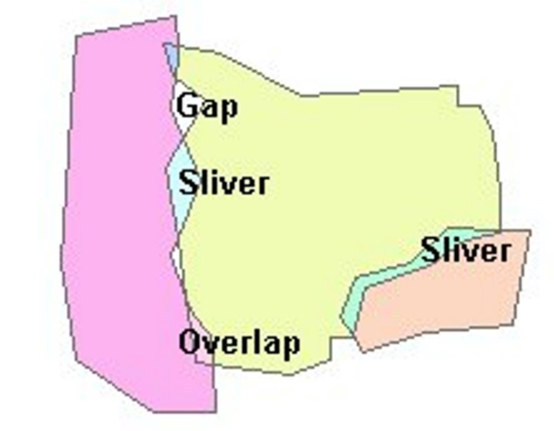
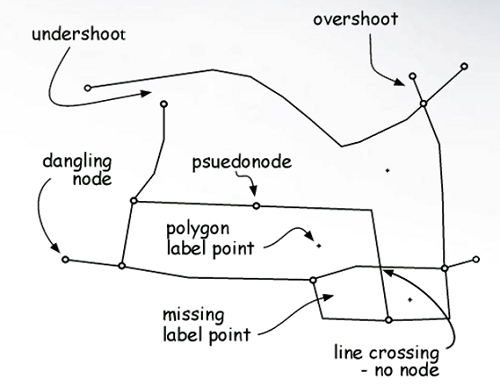
Digitization Errors
Errors that arise when creating vector features:
- Slivers: a feature is created between two features when it should not be.
- Gaps: there should be a feature, but there is not.
- Overlaps: one polygon sits over another polygon.
Digitization Errors
Errors that arise when creating vector features:
- Under/overshoots: vertex misses a connection.
- Extra nodes: unnecessary vertices.
- Missing features: features or attributes missing.
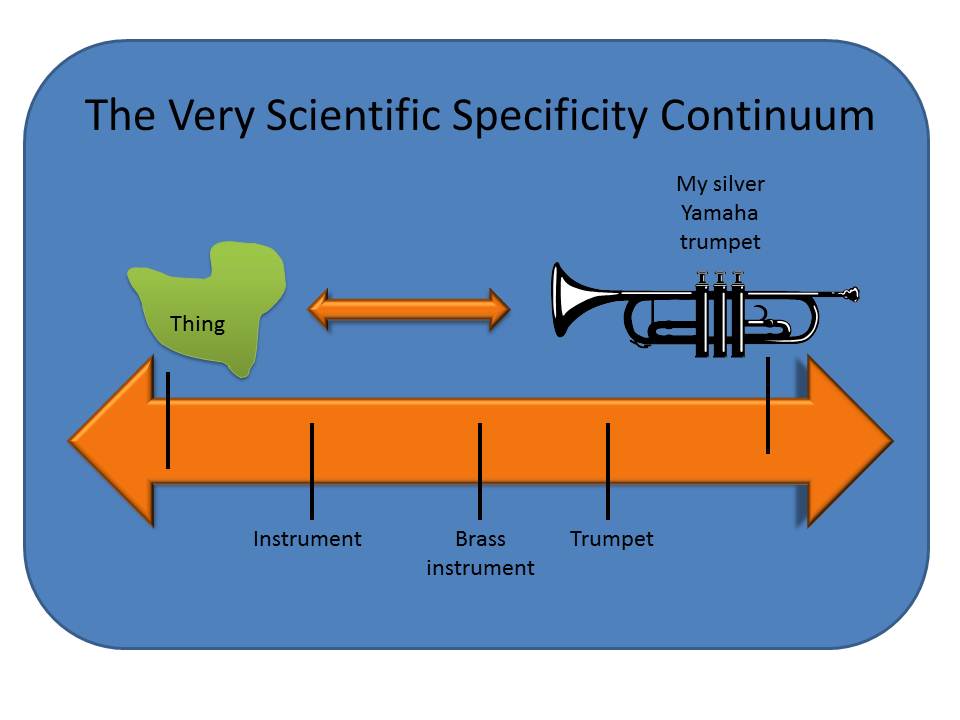
Labels and Boundaries
Since geographic phenomena often don’t have clear, natural units, we are often forced to assign zones and labels in our work (i.e. Census Data).
- A convenient way of simplifying complex processes.
- Often vague and/or ambiguous.
- May be difficult to defend because they are arbitrary.
- Where to draw a boundary and what to call a zone are likely to vary significantly between different people/groups.
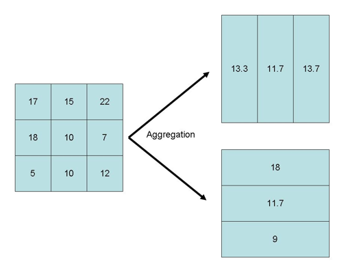
Data Aggregation
Much of the data we use to learn about society is collected in aggregate. We take average values for many individuals within a group or area (i.e. Census Data).
- Lets us explore the general attributes (e.g. mean, median, etc.) for each group/area.
- Compare the attributes between different groups or regions
- Determine the allocation of resources.
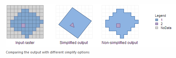
Conversion and Processing
Even with "perfect" data; GIS operations can add uncertainty:
- Re-projecting to different coordinate systems.
- Converting between data types.
- Perform generalizations (i.e. data classification)
Logical Fallacies
A flaw in our reasoning that undermines the logic of our argument.
- Can be made both by accident and on purpose.
- Often lacking evidence to support the claims/decisions made, or evidence is presented in a misleading way.
- “Hasty generalizations” are an example of logical fallacies:
- ‘I saw a violent protester on TV … Protesters are inciting violence.’
Ecological Fallacy
Applying data collected/presented in aggregate for a group/region and applying it to an individual or specific place.
- You cannot make an assumption about individuals within a group based on the aggregate data for that group.
- Census data is averaged for an area, the information about individual values is lost.
- Basically - don't make assumptions about individuals.
Atomistic Fallacy
Occurs when we take aggregated data and aggregate it again at a higher level.
- Take the average income by census DA for the city of Vancouver.
- Average those across the city Vancouver, and you won't get the correct value.
- You are comparing across units of different sizes/populations
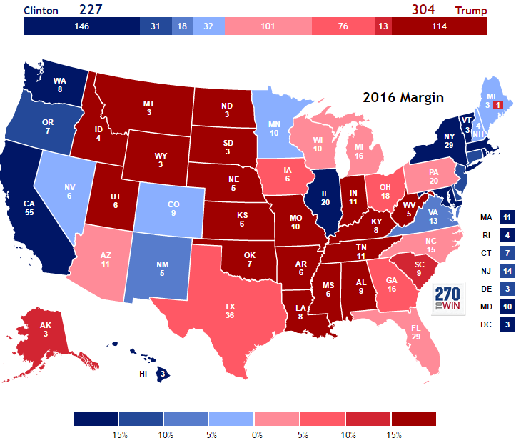
Atomistic Fallacy
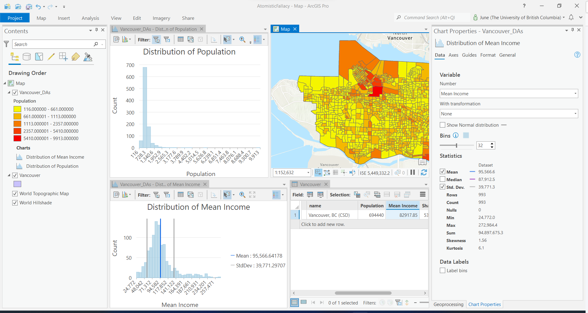
Atomistic Fallacy
The US Electoral College is an example of this in practice:
- Totaling votes per state.
- ... then totaling "delegates" by state.
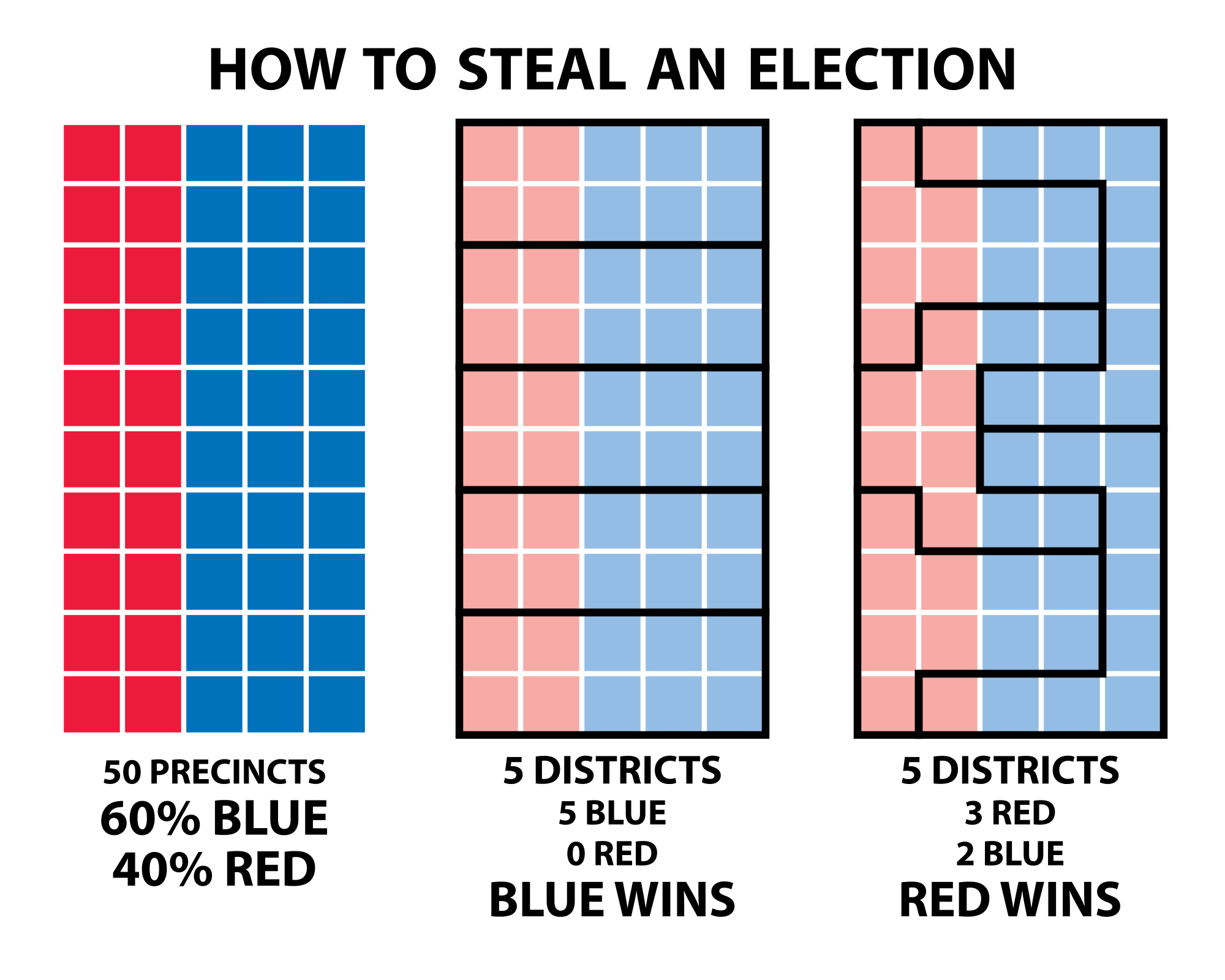
Modifiable Areal Unit Problem
Modifiable, arbitrary boundaries can have a significant impact on descriptive statistics for areas.
- When areas are grouped together, the way you choose to group them can change the values of the groups.
- See this video for more context.
Modifiable Areal Unit Problem
Data collected at a finer level of detail is being combined into larger areas of lower detail that can be manipulated.
- Used to imply things that are not necessarily true.
- Serious ethical implications.
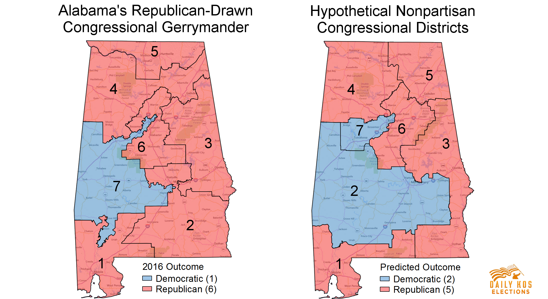
- Gerrymandering is a prime example.
Modifiable Areal Unit Problem
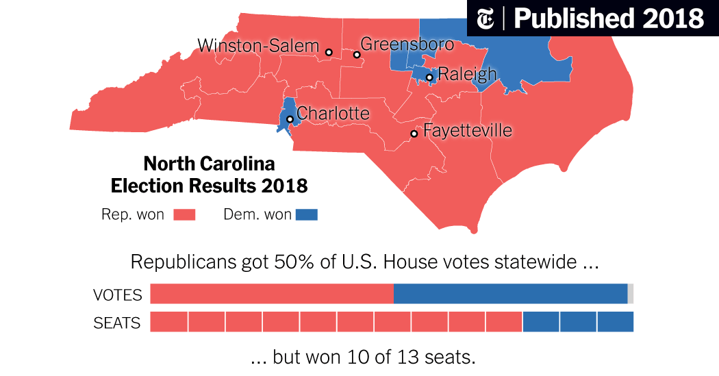
Modifiable Areal Unit Problem
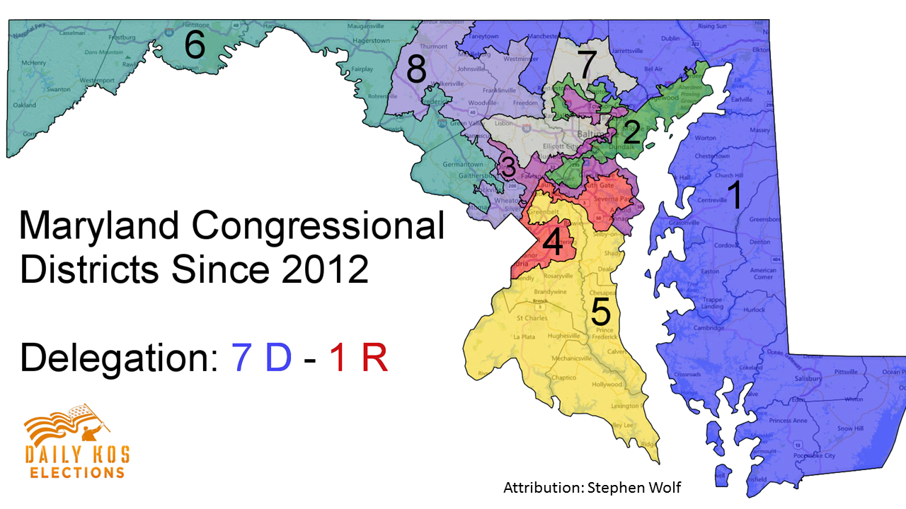
Modifiable Areal Unit Problem
Error Propagation
Errors are cumulative:
- Uncertainty will propagate through the model/system.