| Issue | Solutions |
|---|---|
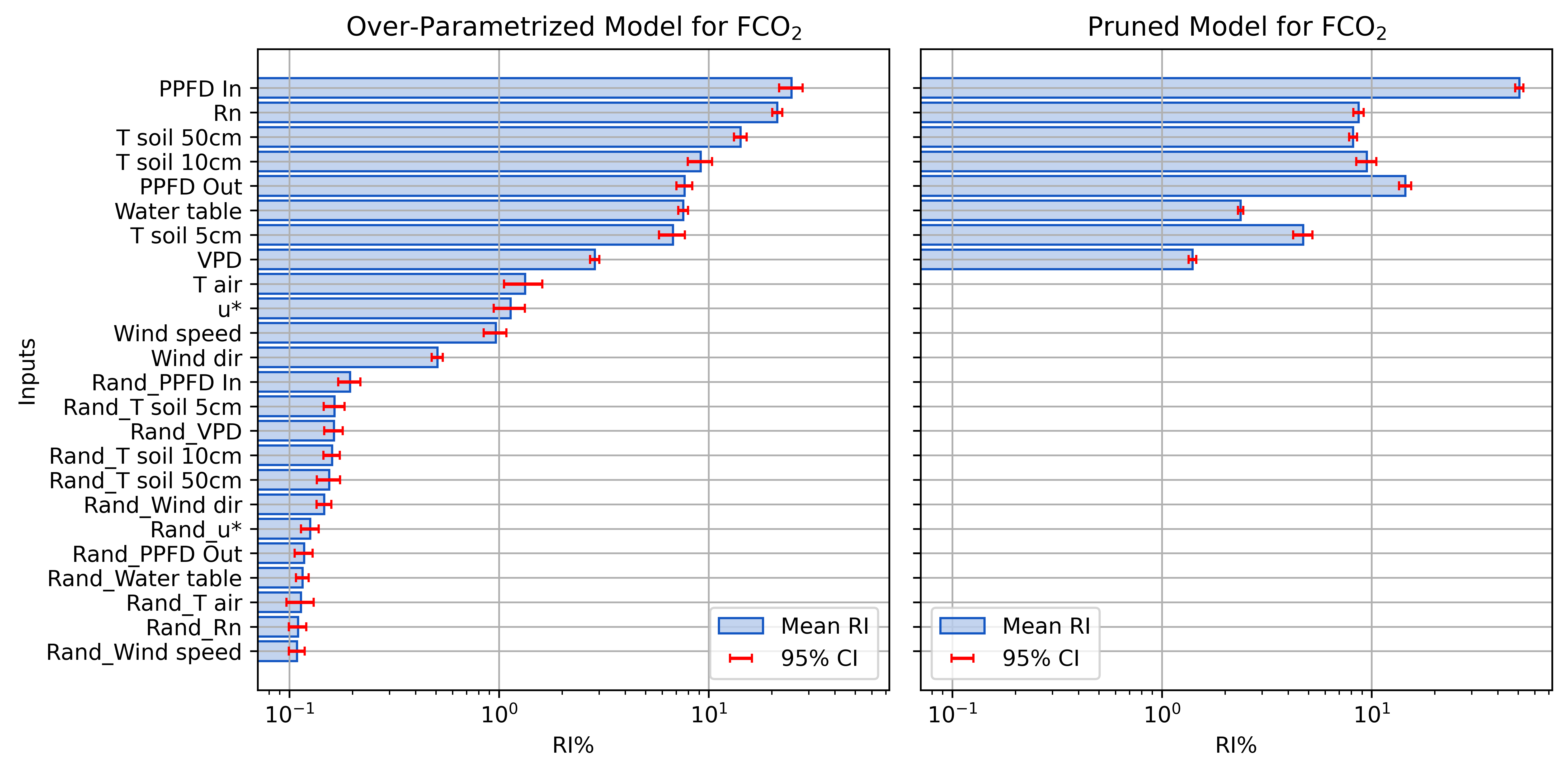
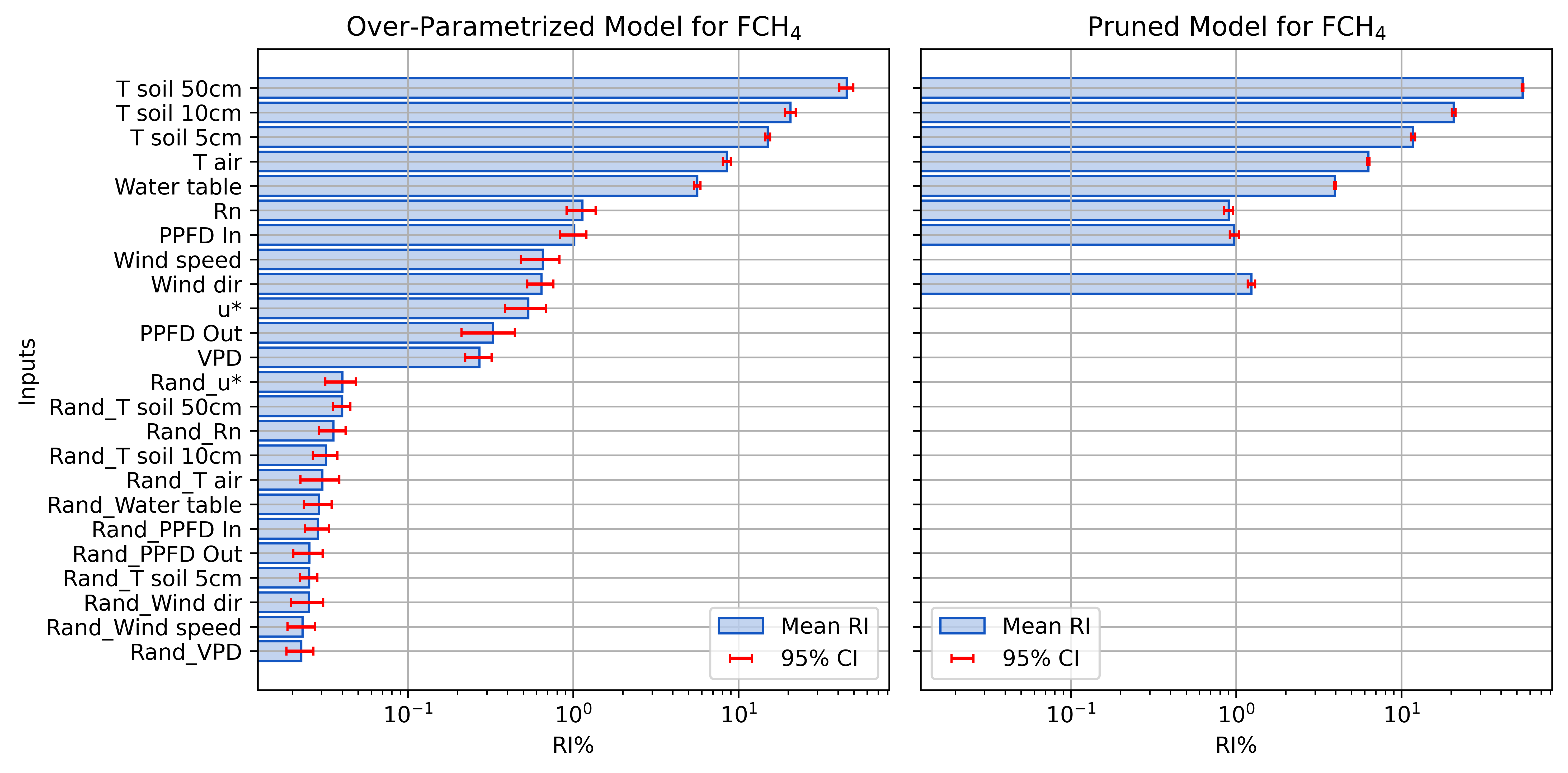
| Over-fitting | - Model ensembles - 3-way cross validation - Pruning inputs |
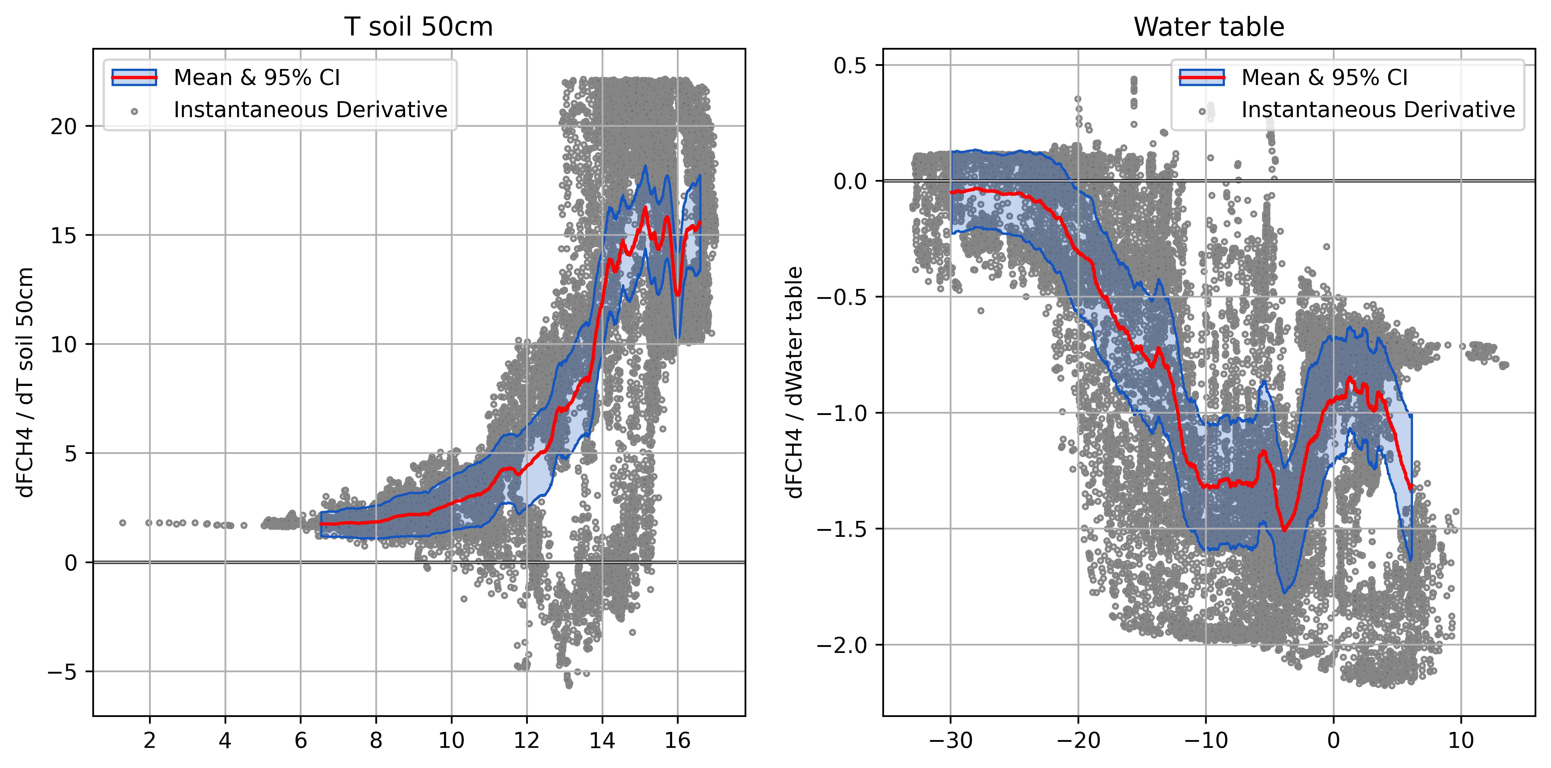
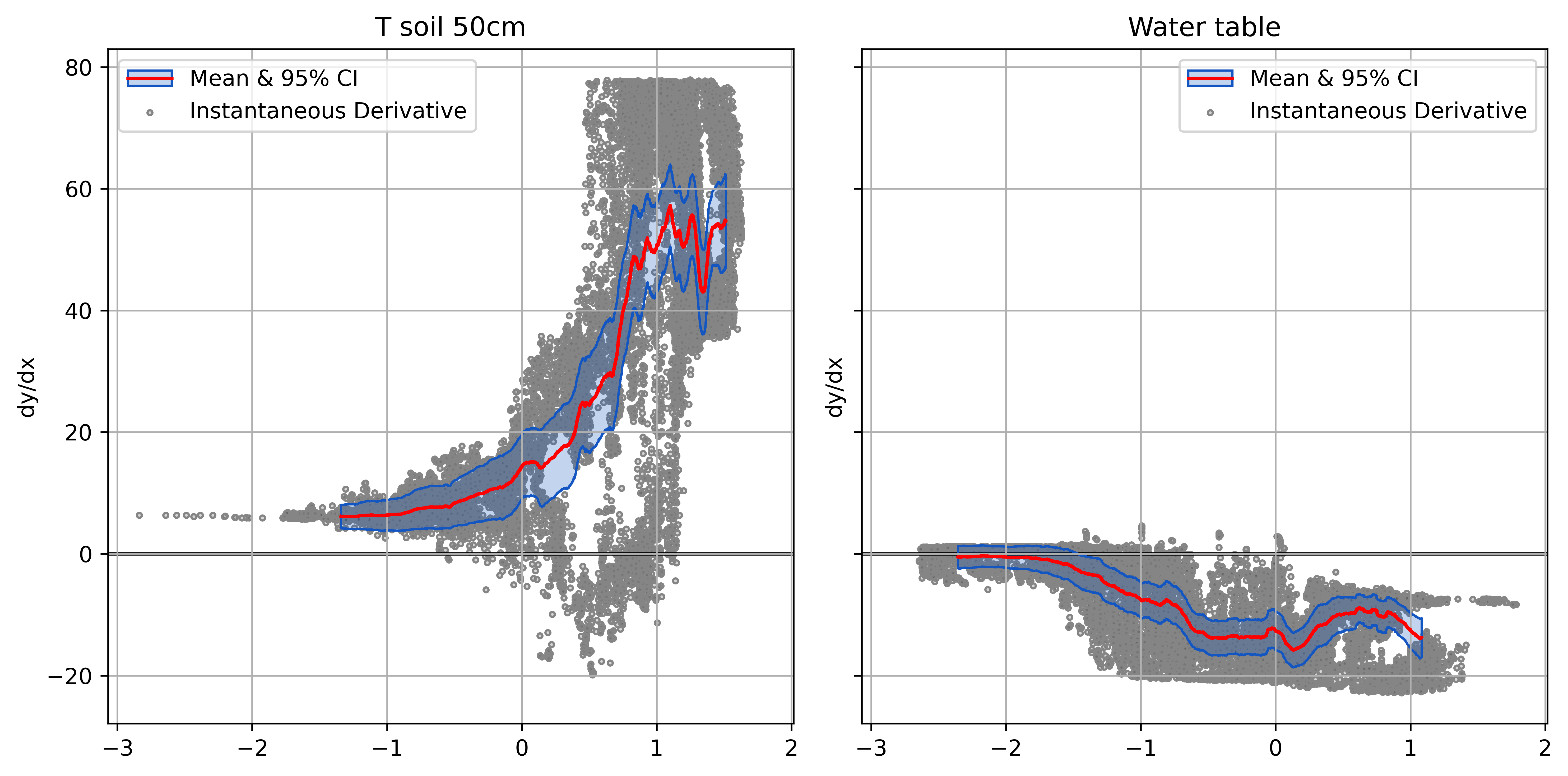
| Black boxes models | - Plot partial derivatives - Feature importance |
| Computationally expensive | - Tensorflow - GPU processing |
Tools and Guidance for Applying Neural Networks to Eddy Covariance Data
Eddy Covariance
Semi-continuous, ecosystem-scale energy, water, and trace gas fluxes.
- Noisy, voluminous data sets
- Frequent gaps
- Observational bias
- Well suited for machine learning!
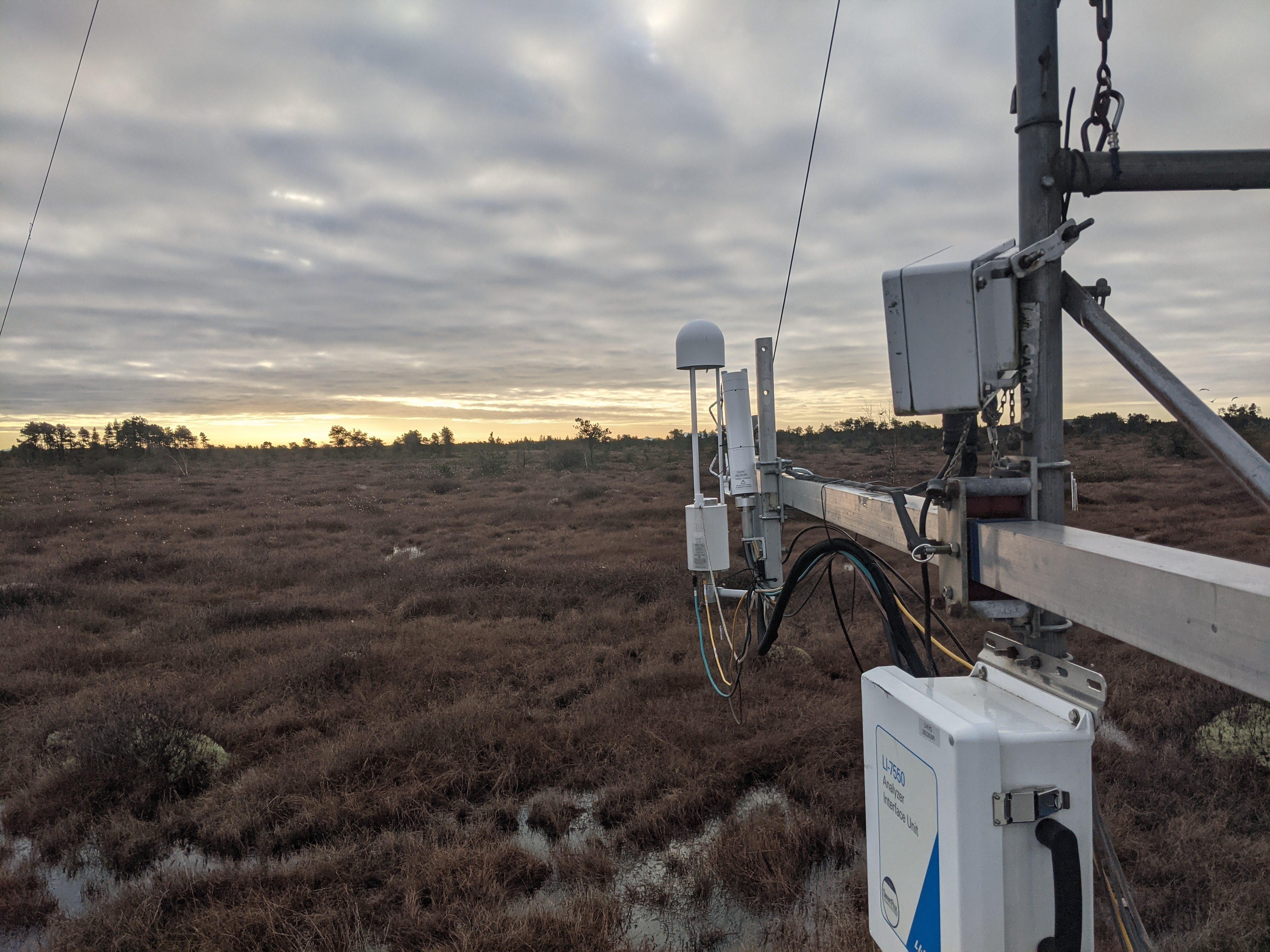
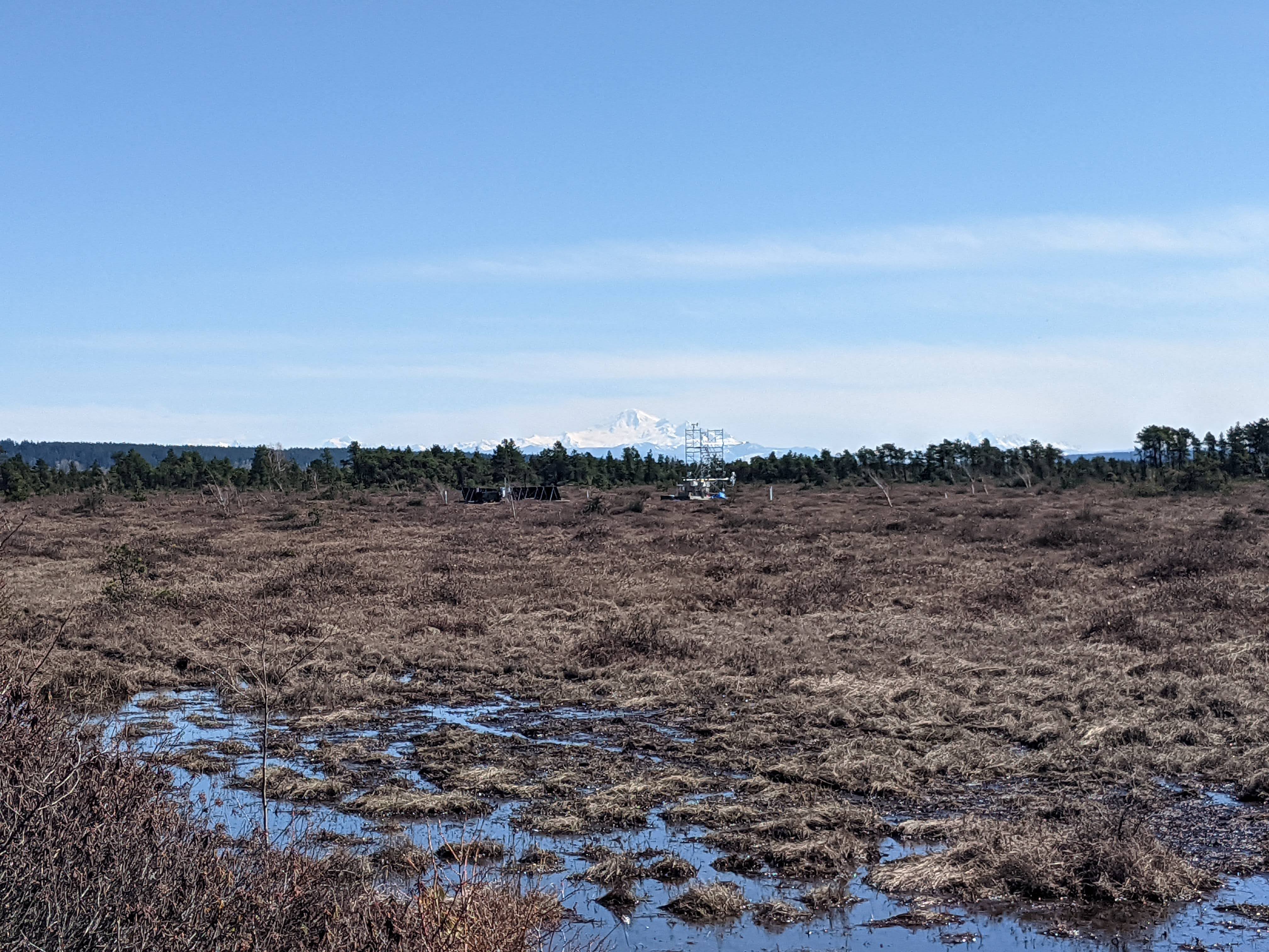
Burns Bog EC Station
Delta, BC
Example Data
Burns Bog EC station
- Harvested peatland undergoing active restoration
- 8+ years of flux data
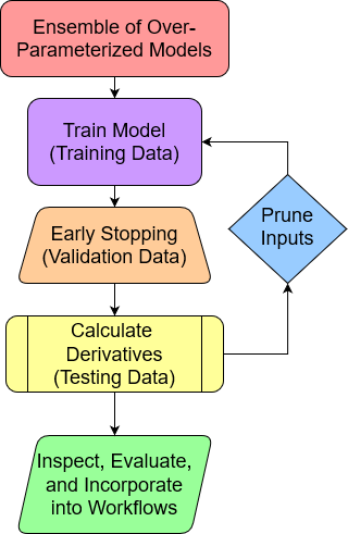
Training Procedures
- Larger ensemble = more robust model
- N \(\leq\) 10 for data exploration/pruning
- Three way cross-validation
- Train/validate/test
- Early Stopping: after e epochs
- e = 2 for pruning stage
Before and After Pruning FCO2
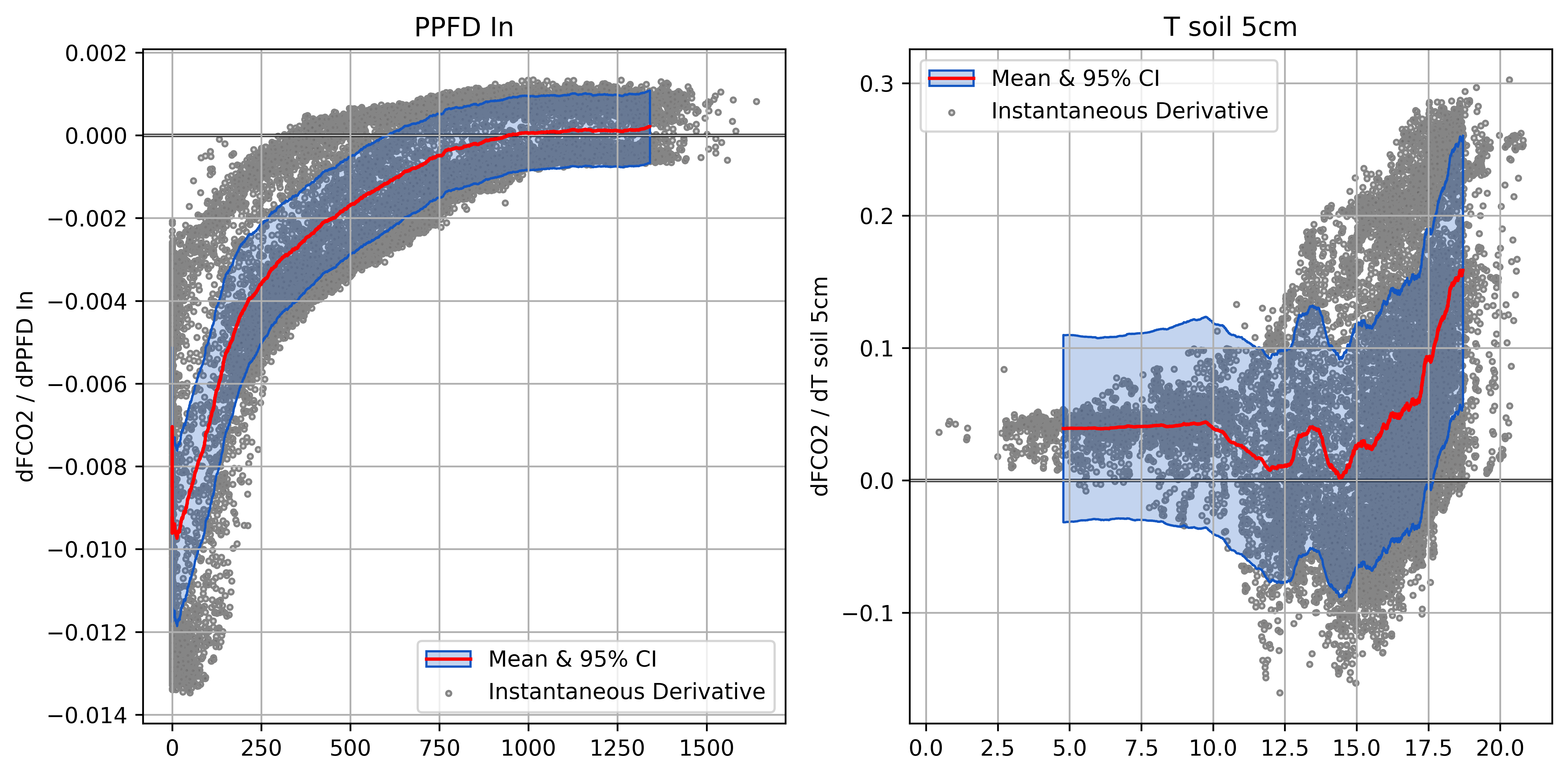
Partial Derivatives of FCO2
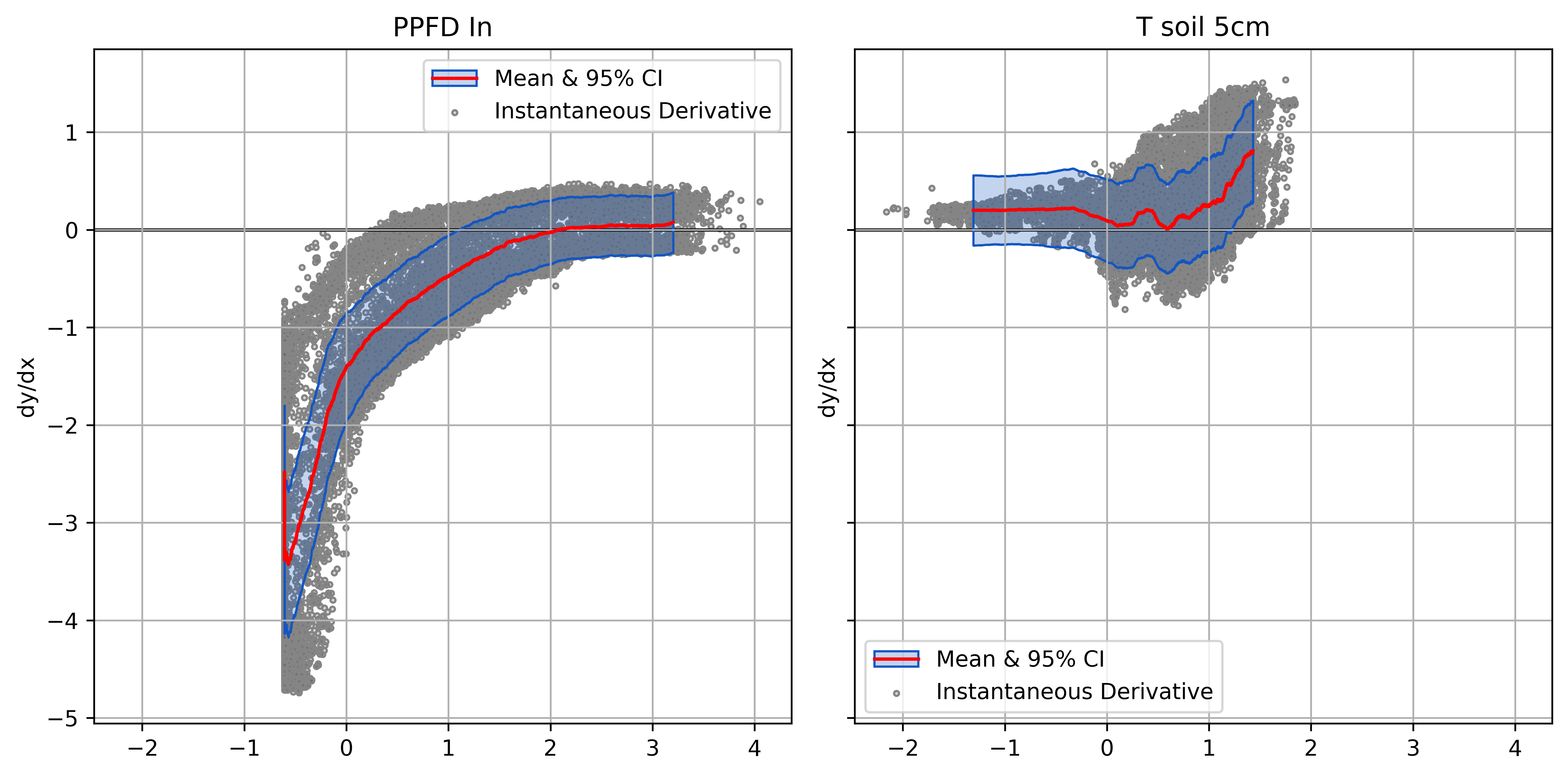
Normalized Derivatives of FCO2
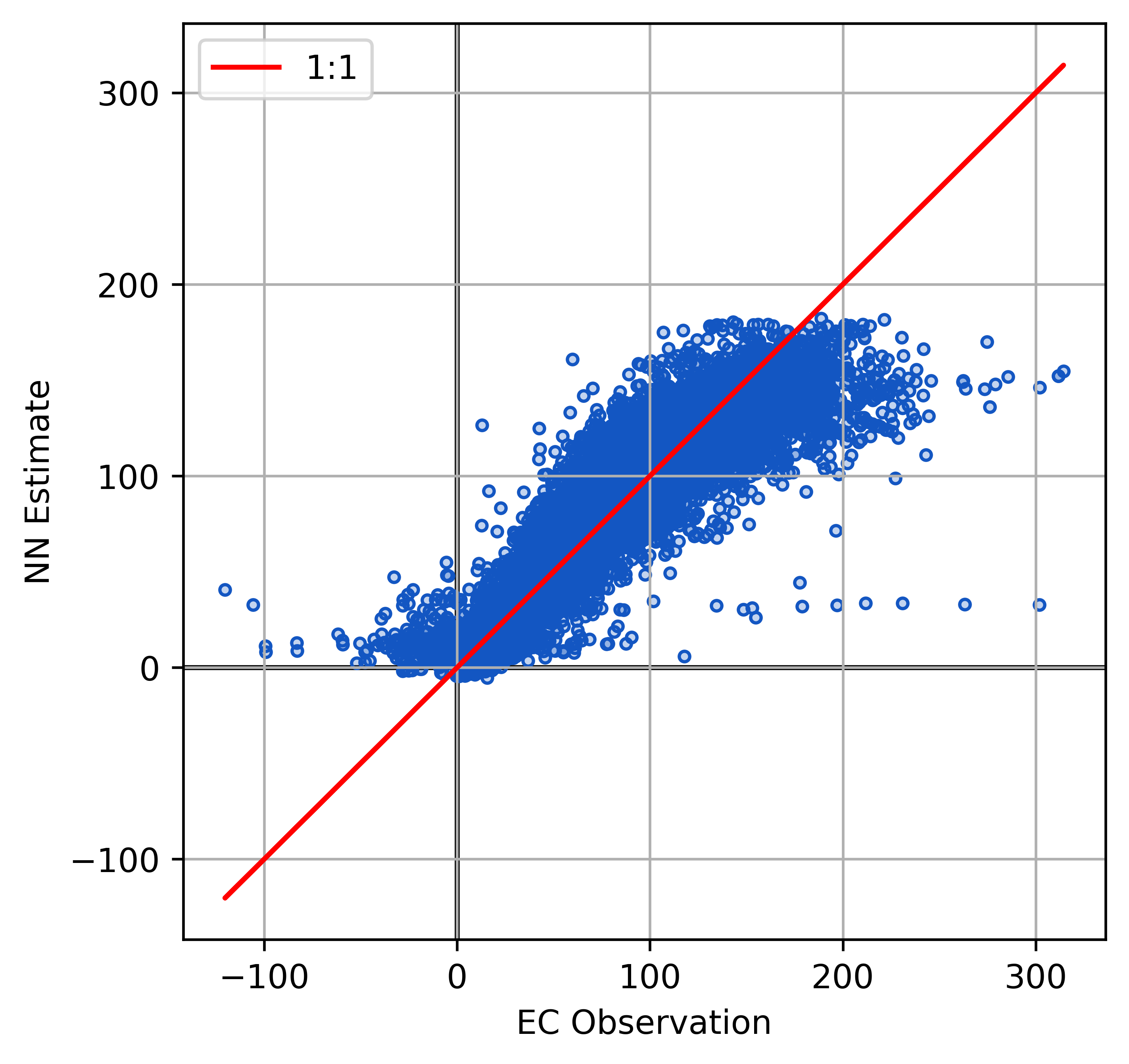
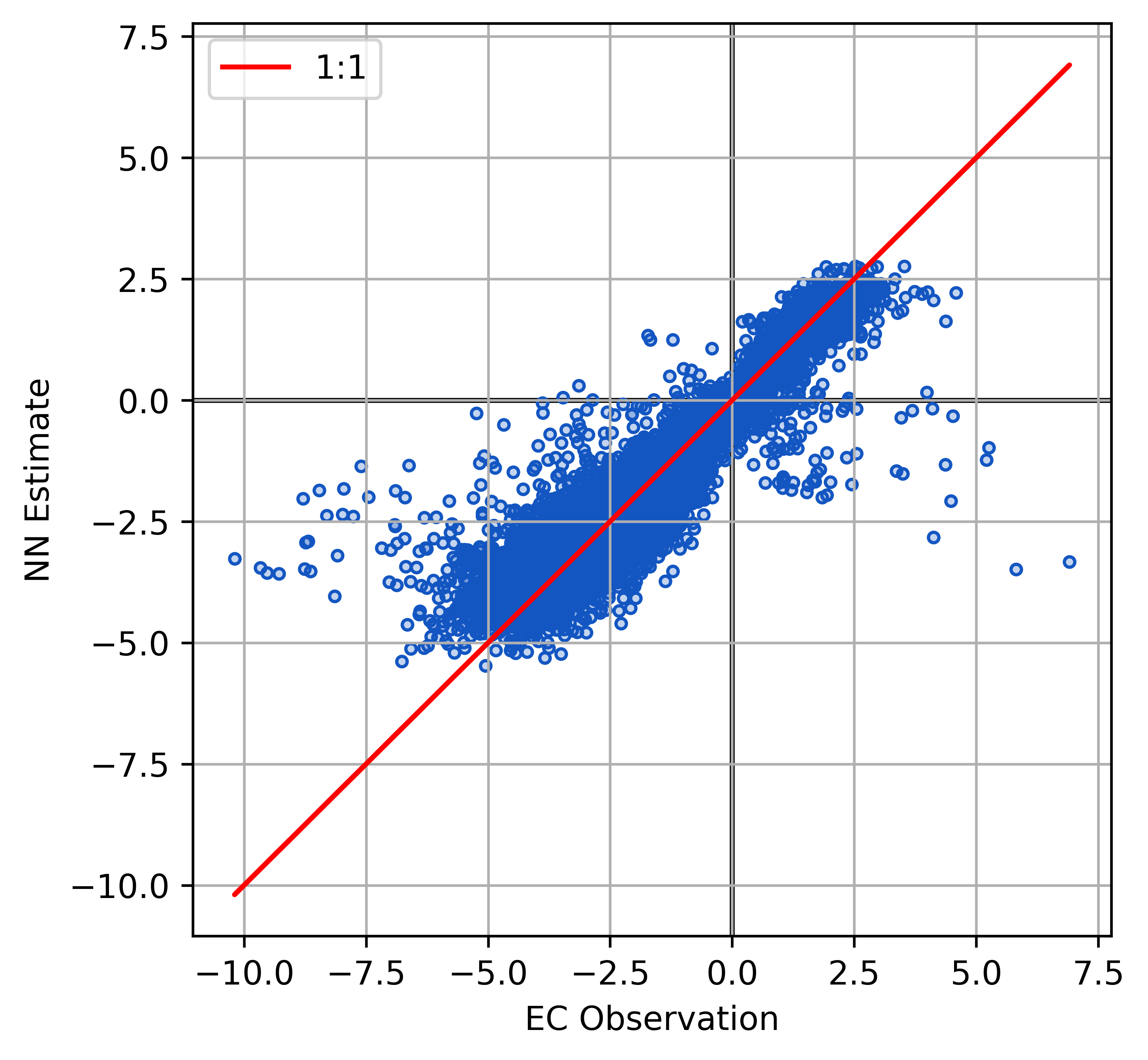
Model Performance FCO2
Plot the model outputs and validation metrics calculated with the test data.
| Metric | Score |
|---|---|
| RMSE | 0.64 \(\mu mol\) \(m^{-2}s^{-1}\) |
| r2 | 0.88 |
Before and After Pruning FCH4
Partial Derivatives of FCH4
Normalized Derivatives of FCH4
Model Performance FCH4
Plot the model outputs and validation metrics calculated with the test data.
| Metric | Score |
|---|---|
| RMSE | 17.17 \(nmol\) \(m^{-2}s^{-1}\) |
| r2 | 0.89 |