Data Classification

Finding patterns in complex datasets, emphasize aspects we think are important.

Descriptive Statistics

When classifying data, descriptive statistics can be used to inform the choice of classification.

They are also frequently used by the classification methods.

Operation	Nominal	Ordinal	Interval	Ratio
Equality	x	x	x	x
Counts/Mode	x	x	x	x
Rank/Order		x	x	x
Median		~	x	x
Add/Subtract			x	x
Mean			x	x
Multiply/Divide				x

Central Tendency

Highlight the central feature in a dataset.

Mode: Most frequent value in a set
Median: Middle value in a set
- Not impacted by outliers - median income
Mean: Sum divided by count
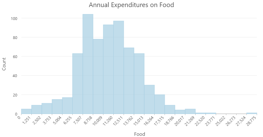
- Impacted by outliers - mean cost of food

Measures of Dispersion

Give context to measures of central tendency.

Range: Difference between maximum and minimum
Interquartile Range: Spread around the median
- Difference between 75th and 25th percentile value - not influenced by outliers
Standard Deviation: Measure of spread around the mean
- $\sigma = \sqrt{\frac{1}{N}\sum_{i=1}^n x_i - U}$ - influenced by outliers

Frequency Distribution

Most useful for categorical data.

Counts per class
Bar charts are a useful way to visualize

Histograms

A useful tool to inspect numeric data

Orders data and bins by intervals
Helpful for classifying data
Outlier detection

Values separated by from the rest of the data

Probability Distribution

Probability of occurrence based on in a quantitative dataset.

Normal Distribution: idealized, based on distance from the mean in standard deviations.

Assumed distribution in many statistical tests.

Deviating from the Norm

Data rarely fits a normal distribution perfectly:

Skew: deviates from a normal distribution

Tails with outliers

Kurtosis: deviates from a normal distribution

Dispersed or clustered

Near Normal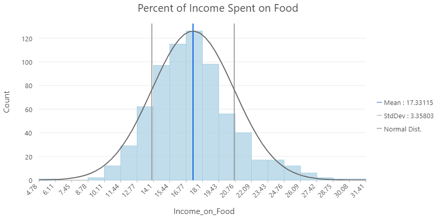

Skewed Normal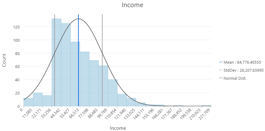

Highly Skewed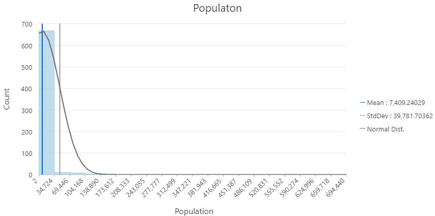

Scaling Data

Often helpful to scale or aggregate a value by a unit of another value - time, area, population etc.

Example: Canada COVID Portal

Total cases aren't useful when comparing vastly different populations
Time rates (rolling 14 day averages) can be smooth out variability.

Normalizing Data

Allows us to account for confounding variables that mask or hide patterns in our data.

Highly correlated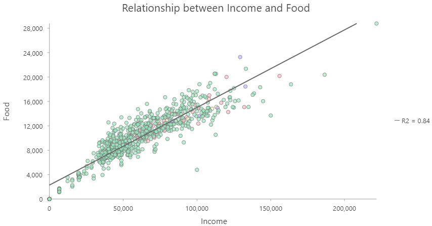

No correlation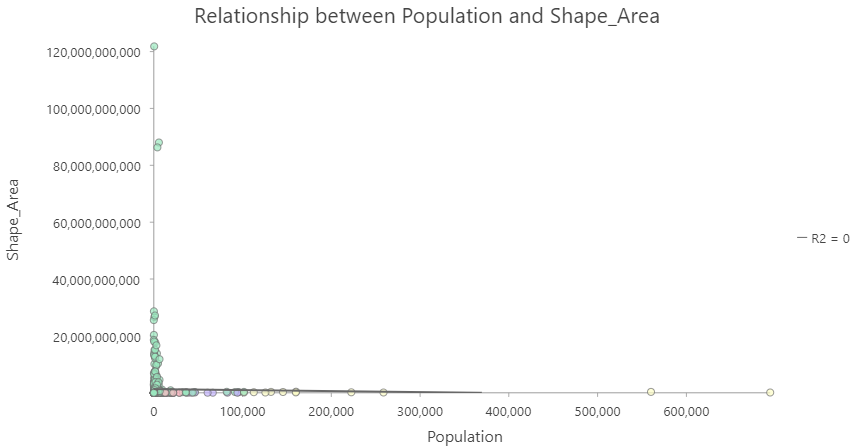

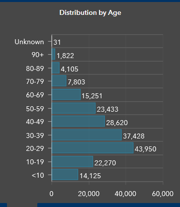
Multiple Factors

It isn't always straightforward to include multiple confounding variables. For example: COVID rates by age groups.

Population by age group
Workforce participation
Occupational exposure

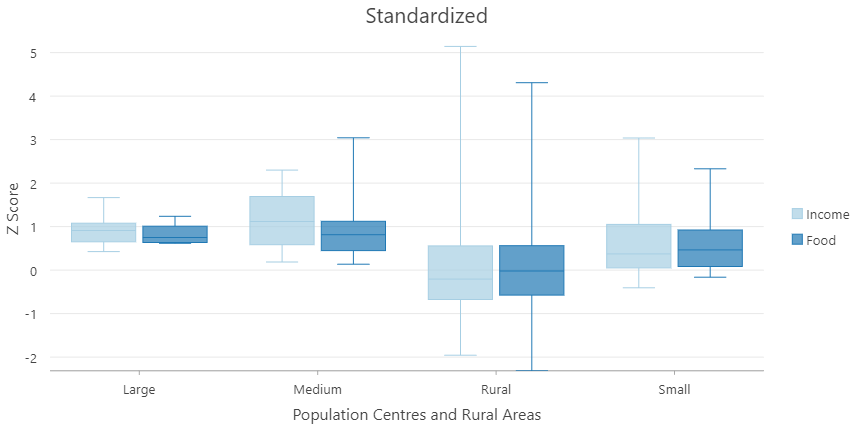
Standardizing

Can also allow us to compare between two or more variables in different units / scales.

$z = \frac{x-\overline{U}}{\sigma}$

Classification Methods

Unsupervised:

Data defined classes - the user decides on the number of classes
The rest is left of up to an algorithm

Supervised:

User defined - the user explicitly defines classes
Or provides set of classes as training data
Degree of user input is variable, more than unsupervised

Common Examples in Arc Pro

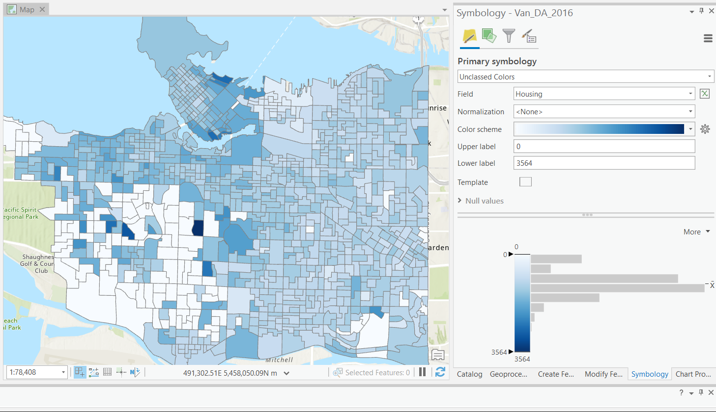
Vancouver dissemination area populations

Not classified
Color scheme is stretched between min/max
Difficult to see patterns

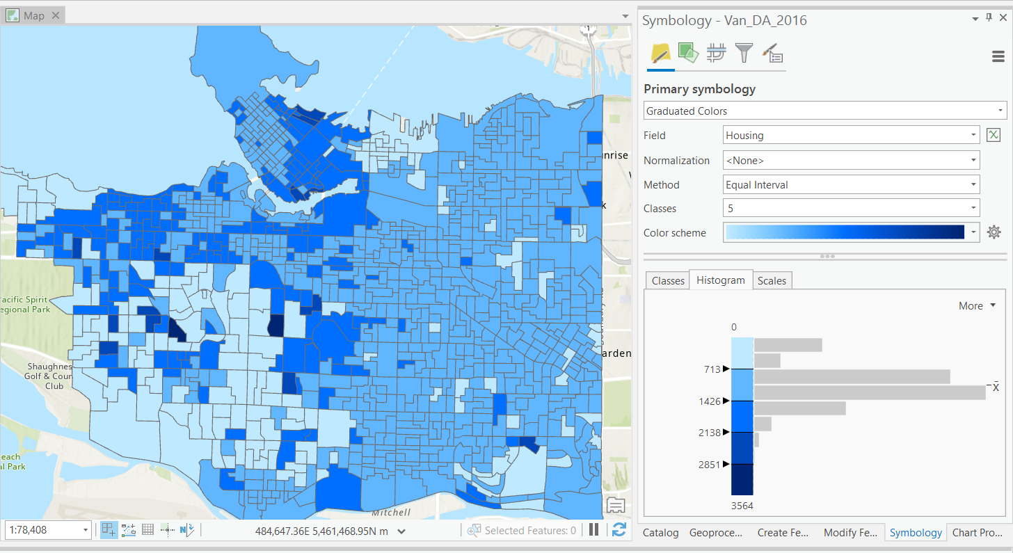
One of the simplest classification schemes.

Data is split to bins of equal width based on the range.
Unsupervised: user defines number of bins.

Equal Interval

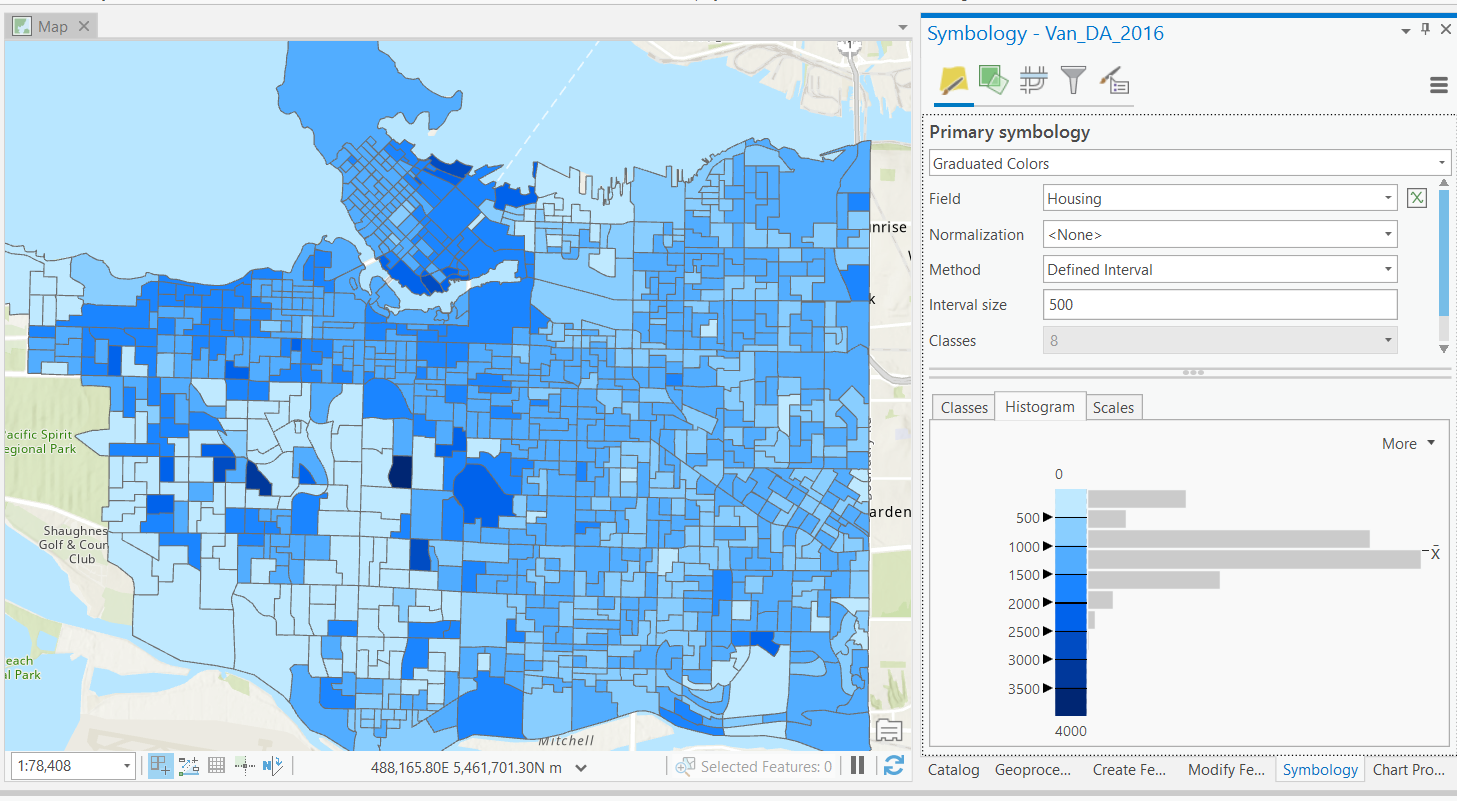
Another of the simplest classification schemes.

Data is split to bins of equal width based on the range.
Unsupervised: user defines bin width.

Defined Interval

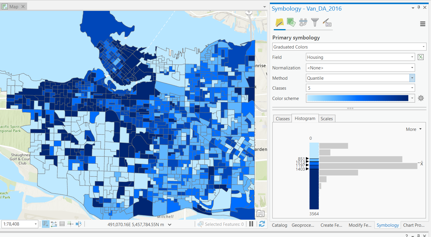
Slightly more complex classification scheme.

Data is split into bins by percentiles.

e.g. 0-20%, 20-40%, ... 80-100%.

Unsupervised: user defines number of bins.

Quantiles

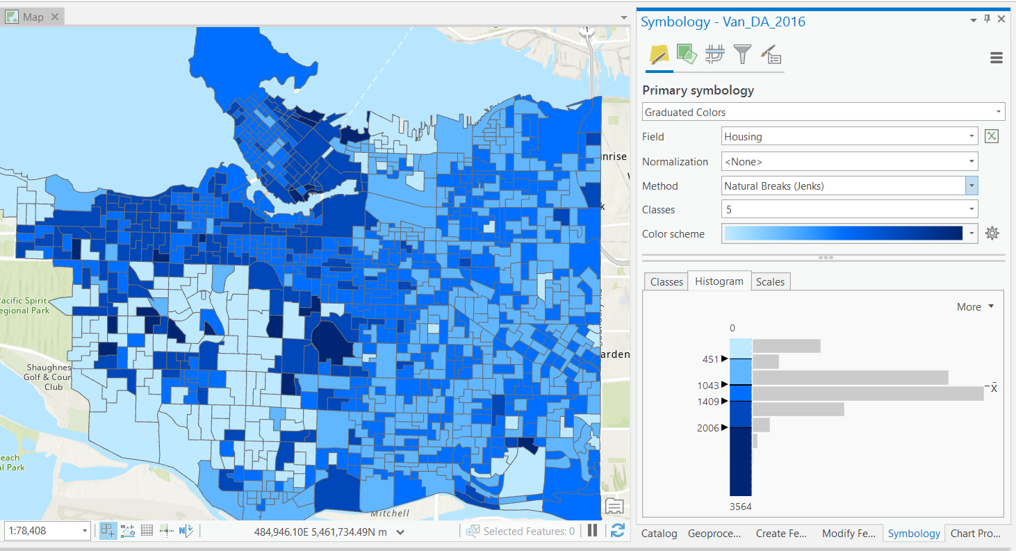
More complex, data is split using the Jenks algorithm.

Optimizes splits, by maximizing within group similarity and between group dissimilarity.

"Natural" classes.

Unsupervised: user defines number of bins.

Natural Breaks

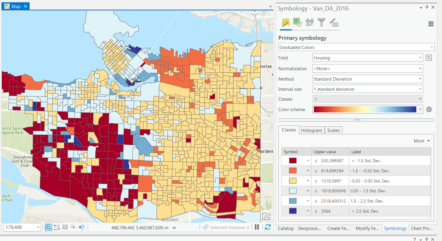
Informative to "experts", not accessible for all.

Distance from the mean in standard deviations.

Unit-less, converts to interval data.
Diverging color maps.

Unsupervised: user defines number of bins.

Standard Deviation

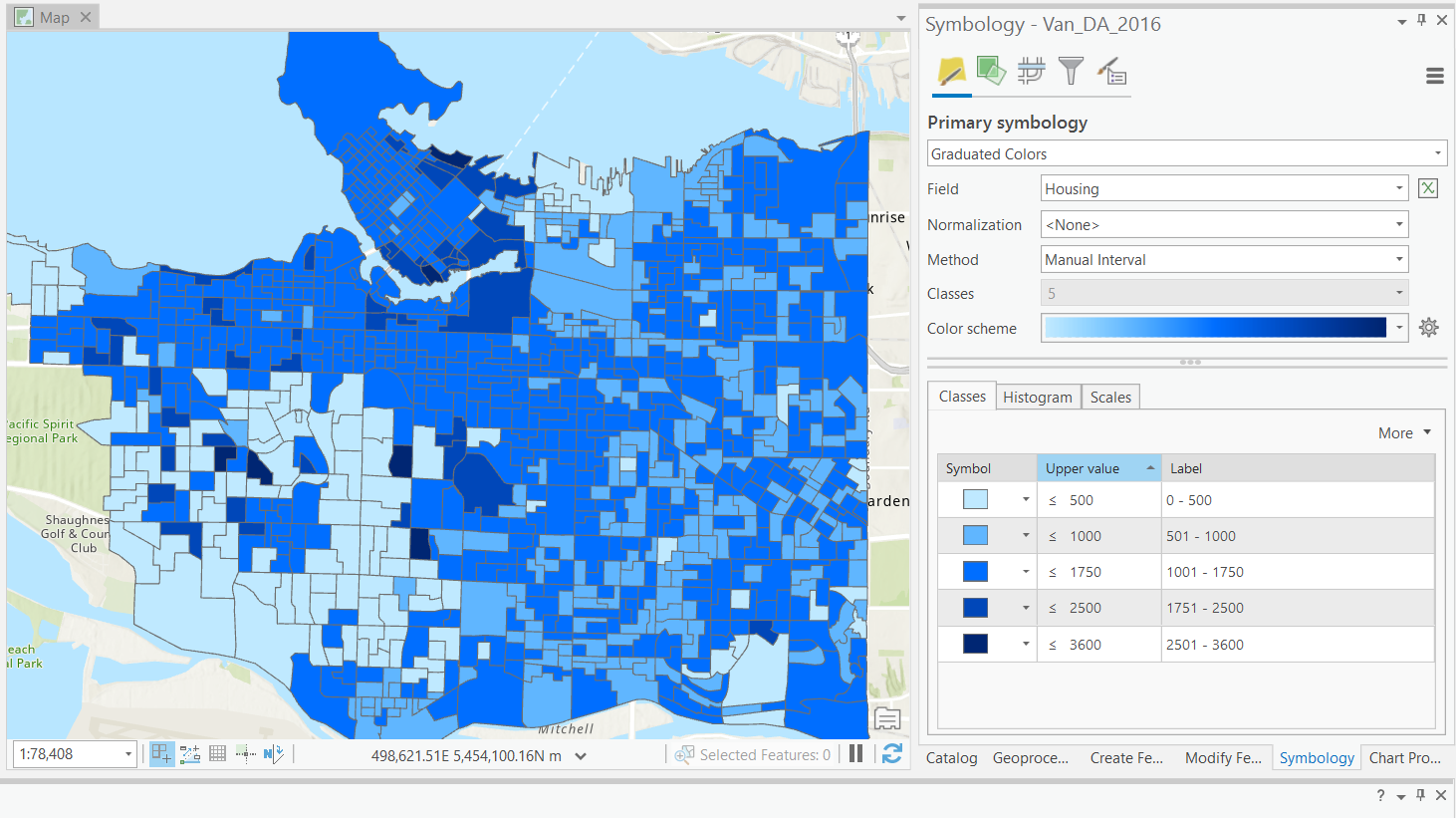
Supervised: User defines break values.

Allows us to choose more meaningful break values if necessary.
Incorporate multiple factors
Influence the way the data is perceived.

Manual Breaks

More Complex Methods

There are many classification methods that are a bit too complex to actually perform in this course.

I'm introducing some because important to be aware of them.
You'll encounter them if you continue with GIS.

K-means

Algorithm uses random steps to group data into clusters.

Unsupervised: user defines number of bins & iterations.

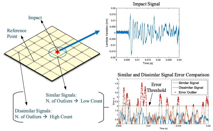
Median Absolute Deviation

Used for automated detection of outliers.

Unsupervised: user defines error threshold.

Median Absolute Deviation

Used for automated detection of outliers.

Unsupervised: user defines error threshold.

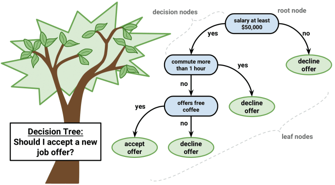
Decision Trees

Fit training data to user defined categories.

Supervised: user provides training classes.
Automated: algorithm determines break values.
Risk of over-fitting

Random Forests

Multiple trees (>100) can be averaged to increase performance and generalization.

Supervised: user provides training classes and "hyperparameters".
Automated: algorithm determines break values.
Low risk of over-fitting

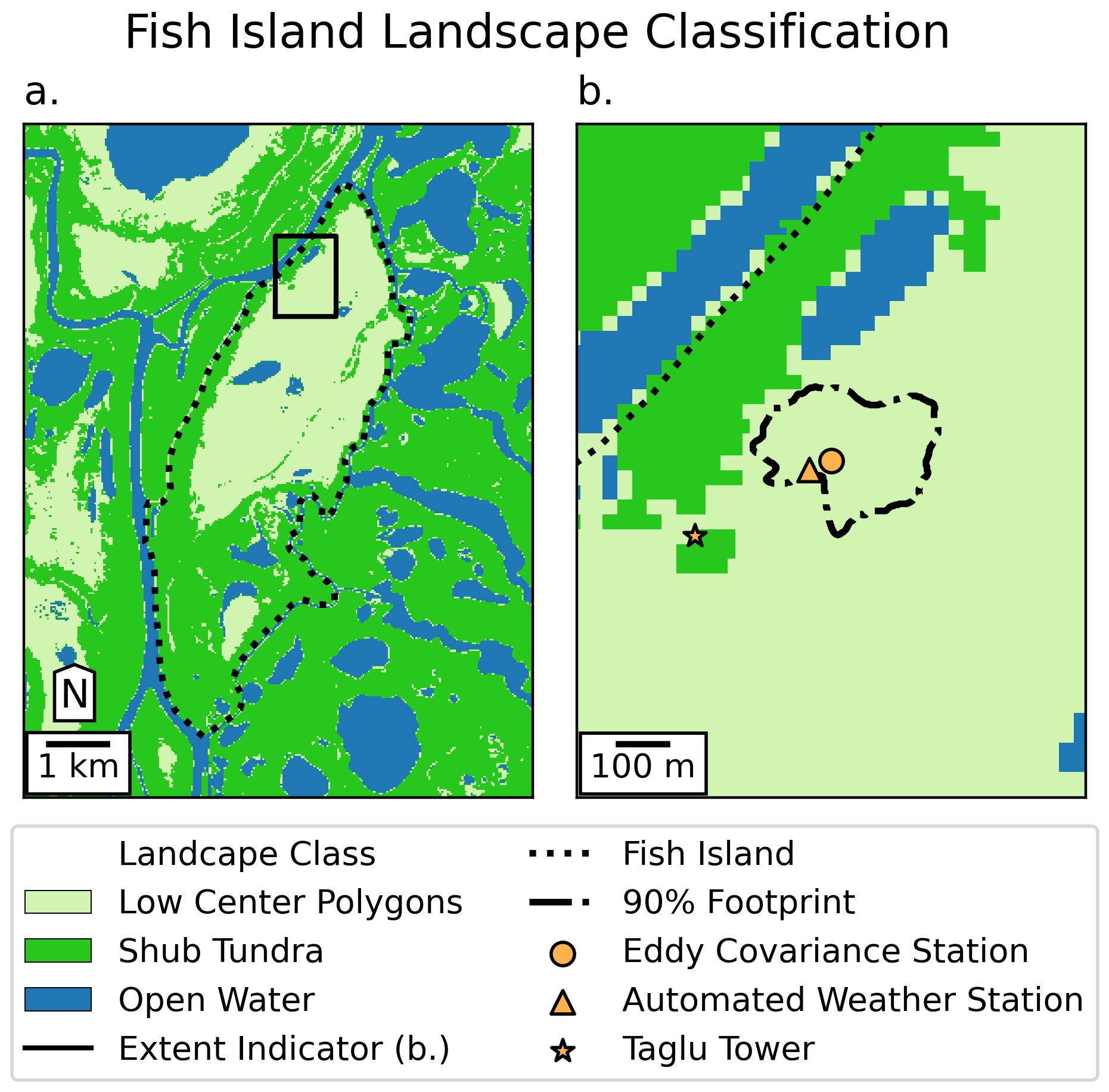
Landscape Classification

Training classes: different ecosystems.
Training data: time series of peak NDVI.
Random forest (100 trees)

96% validation accuracy!

Neural Networks

One of the most complex methods, capable of predictions.

Supervised: user provides training classes and "hyperparameters".
Automated: algorithm maps relationships in dataset.
Risk of over-fitting

Requires careful inspection